ML | Physics-informed neural networks (PINN)
PINN
Physics-informed neural networks (PINNs) represent a significant advancement in the integration of machine learning with physical laws, particularly in the context of solving differential equations. They combine traditional neural network approaches with the constraints provided by known physics, enabling more accurate modeling and predictions in various scientific fields.

Universal Approximation Theorem
Definition
The theorem states that for any continuous function $ f: ^n $ defined on a compact subset of $ ^n $, there exists a neural network $ g $ such that the difference between $ f $ and $ g $ can be made arbitrarily small. Formally, for any $ > 0 $, there exists a neural network with a finite number of neurons such that:
\[ | f(x) - g(x) | < \epsilon \]
for all $ x $ in the domain of interest.
Historical Background
The theorem was independently proven by George Cybenko in 1989, who focused on networks using sigmoid activation functions, and later by Kurt Hornik in 1991, who generalized it to include other activation functions like ReLU (Rectified Linear Unit).
Implications
It has profound implications for the design and understanding of neural networks:
- Expressive Power: It guarantees that neural networks can model complex relationships in data, making them suitable for tasks like image classification, function approximation, and more.
- Architecture Design: The theorem informs users about the necessary architecture (e.g., number of layers and neurons) required to achieve desired approximations.
Limitations
While the UAT provides a theoretical foundation, it does not address practical aspects such as:
- Generalization: The ability of a network to perform well on unseen data is not guaranteed by the theorem alone. Techniques like regularization and cross-validation are necessary to improve generalization.
- Computational Feasibility: The theorem does not specify how to construct the network or find the optimal parameters effectively. In practice, training methods like backpropagation are used, but they may not always reach the global optimum.
Reading
For function alone,
Theorem 2: Suppose that \(U\) is a compact set in \(C[a,b]\), \(f\) is a continuous functional defined on \(U\), and \(\sigma (x)\) is a bounded generalized sigmoidal function, then for any \(\epsilon > 0\), there exist \(m+1\) points $ a = x_0 <...< x_m = b$, a positive integer \(N\) and constants \(c_{ij}, \theta_{ij}, \xi_{ij}\), \(i=1,...,N\), \(j=0,1,...,m\), such that
\[ \begin{align*} | f(u) - \sum_{i=1}^N c_i g ( \sum_{j=0}^m \xi_{ij} u(x_{j}) + \theta_i) | &< \epsilon, \qquad \forall u \in U \\ | f(u) - \sum_{i=1}^N c_i g (\mathbf{\omega_j} \cdot \mathbf{x} + \theta_i) | &< \epsilon, \qquad \forall u \in U \end{align*} \]
Definition and Functionality
PINNs are a type of universal function approximator that incorporates physical laws directly into the training process of neural networks. This is achieved by embedding governing equations, typically expressed as partial differential equations (PDEs), into the loss function of the network. By doing so, PINNs ensure that the solutions generated are consistent with these physical laws, which enhances the robustness and accuracy of the model even when data availability is limited
Training Mechanism
The training of a PINN involves two main components:
- Data Loss: The standard supervised learning approach minimizes the mean squared error (MSE) between predicted outputs and actual data.
- Physics Loss: An additional term is introduced to the loss function that quantifies how well the predicted outputs satisfy the governing physical equations. This is done by computing gradients (using automatic differentiation) at sampled points in space and time, allowing for the evaluation of residuals from the PDEs.
This dual approach allows PINNs to leverage both empirical data and theoretical knowledge, making them particularly effective for problems where data is scarce or noisy.
Challenges and Future Directions
Despite their advantages, PINNs also face challenges:
- Computational Cost: Training PINNs can be computationally intensive, especially when dealing with complex geometries or high-dimensional problems.
- Generalization Limitations: Regular PINNs typically require retraining for different geometries or boundary conditions, which can limit their efficiency in practical applications.
PINN
Key Points on Using Collocation Points in PINNs

It is possible to use collocation points only in Physics-Informed Neural Networks (PINNs). Collocation points are specific locations in the domain where the residuals of the governing equations are evaluated, and they play a crucial role in training PINNs.
Neural networks can indeed be utilized to approximate functions withundetermined parameters, and one of their key advantages is theability to compute various operators, including derivatives and partialderivatives, directly on these networks. This capability isparticularly beneficial in applications like Physics-Informed NeuralNetworks (PINNs), where the derivatives of the network output withrespect to inputs are essential for enforcing physical laws.
神經網路確實可以用來近似具有未確定參數的函數,其主要優點之一是能夠直接在這些神經網路上計算各種運算符,包括導數和偏導數。此功能在物理資訊神經網路(PINN) 等應用中特別有用。
1. Definition and Role
Collocation points serve as the training dataset for PINNs, where the network learns to minimize the residuals of the partial differential equations (PDEs) at these discrete points. The objective is to ensure that the neural network's output satisfies the physical laws represented by these equations at the selected collocation points.
2. Training with Collocation Points
The training process involves minimizing a loss function that combines:
- Data Loss: Measures how well the model fits any available observational data.
- Physics Loss: Enforces that the residuals of the PDEs at the collocation points are minimized.
Using only collocation points can be effective, especially when there is limited observational data. However, it is essential to select these points wisely, as their distribution can significantly affect the accuracy and convergence of the solution. Strategies such as adaptive selection of collocation points based on residual analysis or problem-specific features can enhance performance.
3. Limitations and Considerations
While using collocation points alone is feasible, there are considerations:
- Distribution of Points: A uniform distribution may not capture complex behaviors in certain regions of the domain effectively. Adaptive methods that focus on areas with higher residuals or complexity can improve training efficiency and solution accuracy.
- Generalization: Relying solely on collocation points may limit the model's ability to generalize across different scenarios or boundary conditions unless carefully managed.
In summary, using only collocation points in PINNs is a valid approach, but careful consideration of their selection and distribution is crucial for achieving accurate and reliable results.
Strategies for Selecting Collocation Points
1. Uniform Sampling
- Description: Initially, many PINNs utilize a uniform sampling strategy, distributing collocation points evenly across the domain.
- Limitations: This method may lead to inefficiencies, especially in complex problems where certain regions require more focus due to higher gradients or residuals.
2. Adaptive Sampling Techniques
- Dynamic Adjustment: Adaptive strategies adjust the locations of collocation points during training based on the residuals of the PDEs. This allows the network to concentrate on areas where the solution is more complex or where errors are larger.
- Examples:
- PINNACLE Method: This method dynamically selects collocation and experimental points by analyzing training dynamics and adjusting point locations based on performance metrics. It improves accuracy and convergence speed by focusing on regions with significant residuals.
- Residual-Based Sampling: Points are selected based on the distribution of residuals, with higher densities in areas exhibiting larger errors. This method can involve resampling after a set number of iterations to avoid local minima.
3. Weighting Collocation Points
- Variable Influence: Assign different weights to collocation points based on their importance, allowing the model to focus more on points with higher loss values. This approach helps prioritize learning in critical areas of the solution space.
4. Probability Density Functions (PDFs)
- Guided Distribution: Use information from residuals to create a probability density function that guides the distribution of collocation points. This can lead to a non-uniform distribution that better captures the essential features of the solution.
5. Hybrid Approaches
- Combining fixed and adaptive methods can also be beneficial. For instance, starting with uniformly distributed points and then adapting their locations based on observed performance can provide a balanced approach.
In conclusion, selecting collocation points in PINNs is an iterative process that can significantly impact the model's efficiency and accuracy. Adaptive methods that focus on error distribution and dynamic adjustments during training are particularly effective, as demonstrated by recent advancements like the PINNACLE method. These strategies allow for better representation of complex physical phenomena while optimizing computational resources.
Video
- Steve Brunton
Physics
- Baty, H. (2024). A hands-on introduction to Physics-Informed Neural
Networks for solving partial differential equations with benchmark tests
taken from astrophysics and plasma physics. arXiv preprint
arXiv:2403.00599.
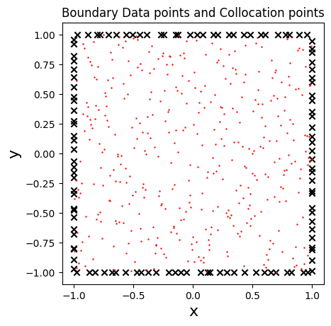
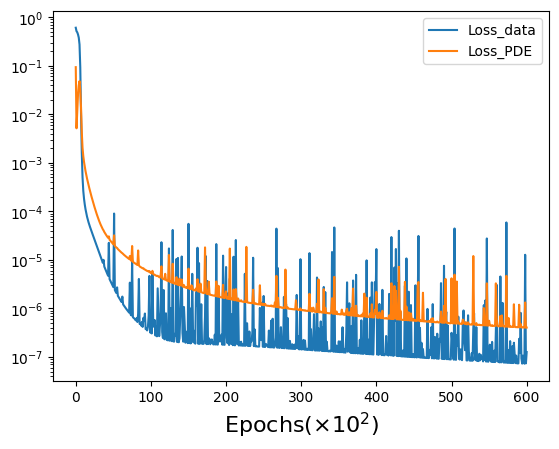
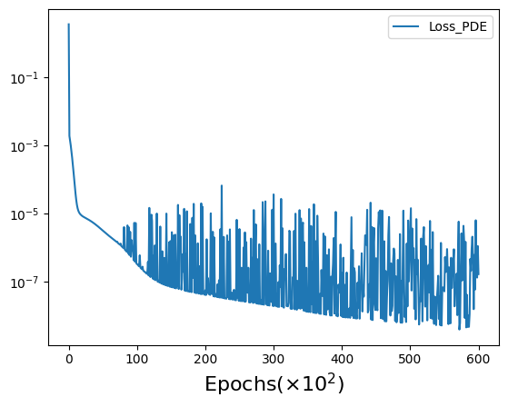
- (Left panel) Distribution of data sets showing the space localization of training data points at the four boundaries (i.e. \(N_{data} = 120\)) and collocation points (i.e. \(N_c = 400\)) inside the domain, for solving Laplace problem using vanilla-PINNs. (Right panel) Evolution of the two partial losses \(L_{data}\) and $L_{PDE} $ as functions of the number of iterations (i.e. epochs).
- Schiassi, Enrico, et al. "Physics-Informed Neural Networks for Optimal Planar Orbit Transfers." Journal of Spacecraft and Rockets (2022): 1-16.
- Barreau, Matthieu, et al. "Physics-informed learning for identification and state reconstruction of traffic density." arXiv preprint arXiv:2103.13852 (2021).
Blog
- 浅谈一下PINN(物理启发神经网络)西南望长安
- PINN的基本原理起源于2017年Prof.George Karniadarkis 组Marziar
Raissi的工作 (2017年已经放在了Arxiv上)
- Physics Informed Deep Learning:Data-driven Solutions of Nonlinear Partial Differential Equations
- 分别用于解决反问题(inverse problem)和正问题(forward problem)
- 正问题和反问题的正经定义可以解释为:正问题,已知原因,根据已有的模型和规律,得到结果状态或者观测,而反问题则是已知结果状态或者观测,来反推原因。
- 反问题我们定义为,已知一些场域内的观测情况,来反推最优的PDE方程的系数/参数的值(这个定义是非常狭隘的和最基本的,后面我们再延申),从某种角度来开,正问题和反问题是一套系统的共生问题
- 神经网络的可微性带来了梯度求解的可行性,而现有的pytorch等框架的autograd带来了工程上实现的便利性
- 正是由于PDE方程已经包含了所有信息(一个世界模型),因此,求解正问题时,PINN完全不需要数据,只需要随意在空间和时间步上采样,然后让PDE方程来评估神经网络的建模是否准确
- PINN的基本原理起源于2017年Prof.George Karniadarkis 组Marziar
Raissi的工作 (2017年已经放在了Arxiv上)
- 内嵌物理知识神经网络(PINN)是个坑吗?
zwqwo
- PINN的原理就是通过训练神经网络来最小化损失函数来近似PDE的求解,所谓的损失函数项包括初始和边界条件的残差项,以及区域中选定点(按传统应该称为"配点")处的偏微分方程残差。训练完成后进行推断(Inference)就可以得到时空点上的值了。
- 特别是用于解决与偏微分方程 (PDE) 相关的各种问题,包括方程求解、参数反演、模型发现、控制与优化等。
- 相比传统微分方程数值求解的描述,这里多出了行式子,也就是对于数据的使用,这也是PINN的特点之一。当然,这三个条件也不一定全都出现,比如边界条件消失,从传统数值方法的角度来看甚至不能满足定解条件。
- 自动微分
- 但PINN这种神经网络不行,即使对于线性方程,也不得不使用非线性求解器(迭代优化器),比如L-BFGS,或者神经网络训练中用得更多的SGD、Adam等。非线性问题的求解通常比线性问题难,这是PINN计算效率上一个避不开的障碍。
- 从这么看来,PINN确实不是太过于新奇的东西。至少在1994年的文献中已经有使用MLP求解二维Poisson方程的例子:
- Dissanayake, M. W. M. G., and Nhan Phan‐Thien. "Neural‐network‐based approximations for solving partial differential equations." communications in Numerical Methods in Engineering 10.3 (1994): 195-201.
- 小结一下以上内容
- 大家都知道PINN是一种(深度)网络,在定义时空区域中给定一个输入点,在训练后在微分方程的该点中产生估计的解。
- 结合对控制方程的嵌入得到残差,利用残差构造损失项就是PINN的一项不太新奇的新奇之处了。本质原理就是将方程(也就是所谓的物理知识)集成到网络中,并使用来自控制方程的残差项来构造损失函数,由该项作为惩罚项来限制可行解的空间。
- 用PINN来求解方程并不需要有标签的数据,比如先前模拟或实验的结果。从这个角度,对PINN 在深度学习中的地位进行定位的话,大概是处于无监督、自监督、半监督或者弱监督的地位,这几个不尽相同的说法在不同语境下都有文献提过。
- PINN算法本质上是一种无网格技术,通过将直接求解控制方程的问题转换为损失函数的优化问题来找到偏微分方程解。
- 如果把PINN当作是单纯的数值求解器,通常来讲,不管从速度或者精度,PINN在性能上并不能跟传统方法(有限差分、有限元、有限体积等大类方法)抗衡。(not sure)
- “内嵌物理”(Physics informed)对于科学机器学习的必要性。值得一提的是,内嵌物理知识神经网络并不是一种作为数据驱动方法对立面的、单纯的“知识驱动”方法,而是作为数据方法与传统知识驱动方程的桥梁存在,也就是“知识”和“数据”共同驱动的方法
- 这节对一个不是太简单的方程进行了数值求解,但解方程其实也并不是PINN的主业。当然,对于PINN而言,解方程这种“正问题”跟参数发现等这些“逆问题”在求解形式上没有太大区别,能比较好求解“正问题”的PINN方法对于“逆问题”也会有不错的表现。
- CFD与其说是计算科学,更像是一门实验科学,需要物理实验数据来对解算的模型进行验证,还面临诸多困难。
- 在工程模型中,可能还涉及逆问题的求解,也就是边界条件和流体的各种参数未知的情形下,如何通过部分测量数据得到精确的模型参数和流场的重构。
- CFD网格质量对结果的影响比较大,计算中网格划分本身也是非常耗时的。最后,目前的CFD软件都非常庞大,比如OpenFoam,对每一类问题都有专门的求解模块,拥有超过10万行的科学计算代码,其更新与维护也是一件难事。
- 刚好,PINN有部分解决以上问题的能力。PINN对各种数据的融合是非常自然的,不管是压强标量场的时空散点数据、速度矢量场的时空散点数据,还是示踪粒子的运动轨迹,都可以非常容易地融合到PINN的求解中。
- 对于PINN来讲,求解正问题与求解包含数据的逆问题在形式上并没有太大区别,这是它的巨大优势之一。
- 即在时空散点测量数据比较充足的情况下,进行CFD相关的参数估计、流场重建、代理模型构建等问题的求解。与传统的CFD求解器相比,PINN在集成数据(流量的观测值)和物理知识(其实就是描述该物理现象的控制方程)方面更胜一筹。
- 比较直接的是通过速度观测来重建全流场。在气动力学等学科的实验研究中,可以利用光学设备,通过粒子图像测速(Particle Image Velocimetry,PIV)和Particle Tracking Velocimetry(PTV)方法测量的得到多个散点速度。然而散点速度并不能满足需求,高分辨率的速度场对于可视化和后续分析是必不可少的。一个非常自然的想法就是通过类似图像插值来实现从散点到高分辨率流场的“超分辨”,但是这种方式处理得到的结果可能“并不符合物理规律”。作为融合了物理知识的PINN方法,可以非常自然地从这些稀疏速度信息来重建分辨率的整体速度场。
- 连初值和边界条件都不需要。这种适合PINN建模求解的逆问题对于传统的CFD求解器来说并不是一件容易的事情。
- PINN的优势不再正问题求解上的速度和精度,而是在于融合数据和知识。
- PINN还有研究的必要吗?AI4Science探索
- PINN即内嵌物理知识神经网络,该领域更广泛、通用叫法应该是物理驱动的神经网络(深度学习),刚接触到物理驱动的神经学习方法时,总会有一些疑惑:物理驱动的深度学习方法在求解一些物理系统(由物理方程所描述控制的系统)时,需要已知一些物理信息如偏微分方程。但传统数值方法发展这么多年了,如有限差分、有限体积方法已经非常成熟,也成功用于物理系统的求解,求解准确性非常高。但是物理驱动的深度学习如神经网络方法
- 相比于传统数值方法有以下潜在优势:
- 反问题计算上有比较大的优势。传统数值方法主要针对复杂问题的正计算,如已知边界条件、已知控制方程下的正计算,优势非常强。相比之下,在正计算问题上,深度学习方法逊色一些。但针对一些反问题,如已知一些测量数据和部分物理 (方程中某些参数未知、边界条件未知),深度学习方法可以形成数据和物理双驱动的模型,比基于传统数值方法去做数据同化(data assimilation)效率更高。
- 需要做快速推断时,优势更明显。一方面,当面对一些数值问题,可以不需要熟悉数值方法背景(不必利用数值格式去推导求解),可以直接利用加物理损失的方法得到一个参考解;另一方面,当问题边界需要不停地换,或者很多源需要不停的变化的问题设定下,如果利用大量时间去训练一个网络,如利用lulu老师提出deeponet方法(物理驱动的神经网络方法),在推断阶段就能实现快速预测。高维问题上的潜在优势。
- 神经网络确实能处理许多高维问题,但很难说神经网络方法在一些benchmark问题上已经完全超越了传统问题,还需要进一步讨论。
- 一GAN崩了不听话的PINN
| 2025年01月27日 西南望长安
- 这篇论文是关于如何使用GAN来自适应调整PINN的损失函数,从而让PINN 收敛到更好的性能。论文题目是“DEQGAN: Learning the Loss Function for PINNs with Generative Adversarial Networks”
- 当我们把PINN用在实际工作中,你会发现有时候很难搞到收敛的结果,把PINN 当作一个所谓的physics solver似乎只是一个镜花水月的梦想。why? 首先,神经网络的自由度远远超出了pde方程的复杂度,这就像是高维生物在看低微生物,亦或者人类在看小蚂蚁,有无数种方法可以玩弄小蚂蚁,所以虽然pde只有一个解,但是神经网络有一万条路去拟合,其中大部分都跑到了局部最优
- 典型做法是这样的,大家不停试错,为这些损失函数配置权重,最终找到一组可以让模型收敛,论文里“trail and error”三个词可能代表了科研民工们三个月的工作量。但是这样的人肉优化是不是最好的,我不置可否,虽然它很artificial,但好像不咋intelligence。
- 更有甚者,就是直接拿一堆样本把模型都监督学习跑了几万个epoch训好了,然后拿pde loss“辛辛苦苦的”跑了三个epoch;亦或者给监督损失一个极大的权重,pde一个忽略不计的权重。这仿佛去吃牛肉面,只看到了牛肉沫,剩下的全是科技狠活出来的牛肉味儿。
- 说起来简单,其实GAN 也不是什么灵丹妙药,毕竟GAN自身就是天下一等一的不稳定,难训练。
- 如果大家去看论文里下表的参差不齐的学习率设计,你就知道作者为了把它调收敛也是花了不少心思,但是好在GAN的理论研究比较多,怎么把GAN 搞收敛已经有比较多的手段了。
governing equations from scarce data
- Chen, Z., Liu, Y., & Sun, H. (2021). Physics-informed learning
of governing equations from scarce data. Nature communications, 12(1),
6136.
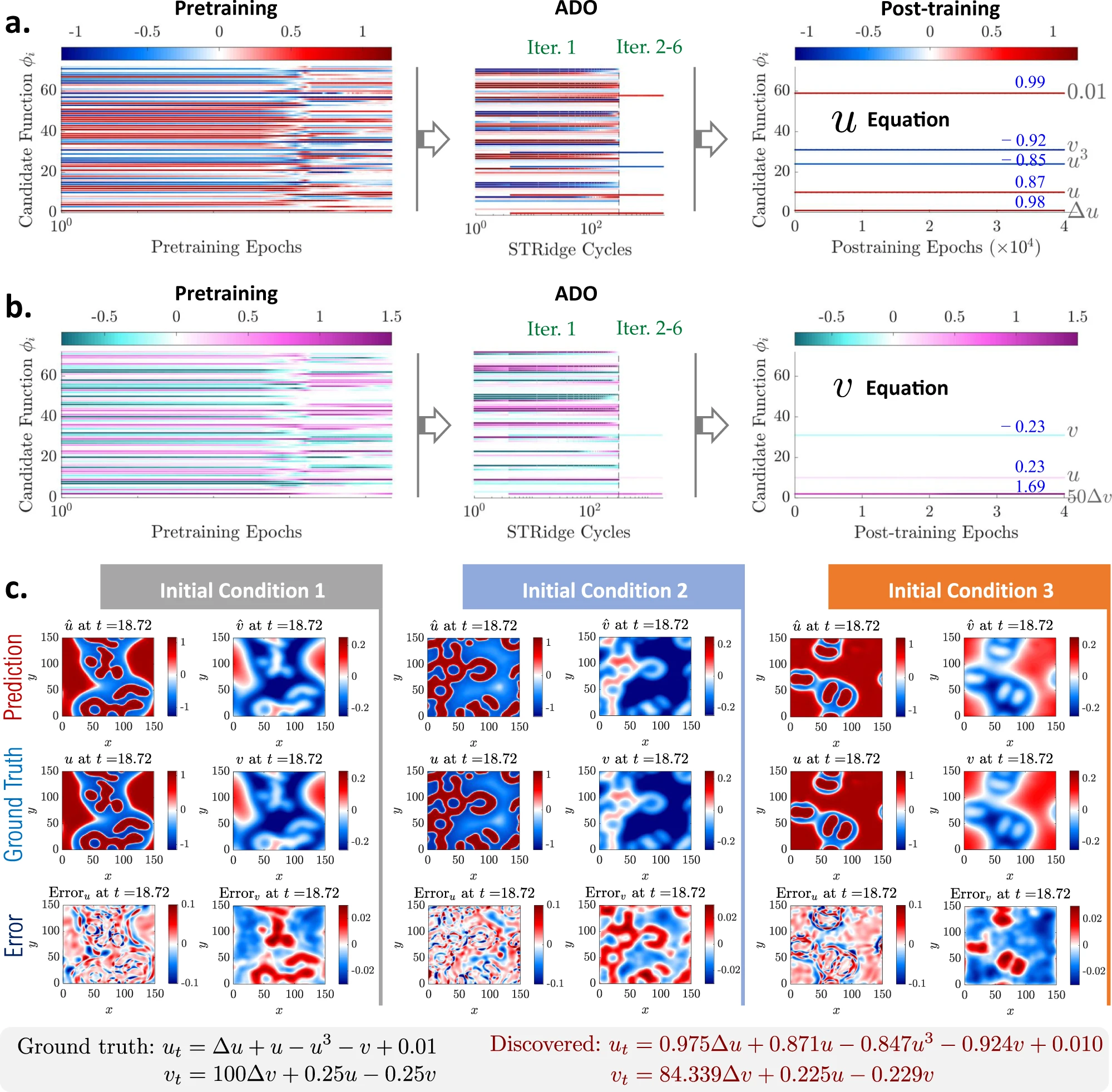
- 通过数据发现描述复杂物理系统的控制方程或规律,可以极大地促进各个科学和工程领域对这些系统的建模、仿真和理解。本文提出了一种新颖的方法,称为稀疏回归的物理启发神经网络,用于从稀疏和噪声数据中发现非线性时空系统的控制偏微分方程。特别地,该发现方法无缝集成了深度神经网络在丰富表示学习、物理嵌入、自动微分和稀疏回归方面的优势,以逼近系统变量的解,计算必要的导数,以及识别形成方程结构和显式表达式的关键导数项和参数。该方法的有效性和鲁棒性在多种偏微分方程系统的数值和实验上得到了验证,这些系统考虑了不同的数据稀缺性和噪声水平,以及不同的初始/边界条件。所得的计算框架显示了在大规模准确数据难以获取的实际应用中发现封闭形式模型的潜力。
Generalization of PINNs
References
- Dissanayake, M. W. M. G., and Nhan Phan‐Thien. "Neural‐network‐based approximations for solving partial differential equations." communications in Numerical Methods in Engineering 10.3 (1994): 195-201.
- Raissi, Maziar, Paris Perdikaris, and George Em Karniadakis. "Physics informed deep learning (part i): Data-driven solutions of nonlinear partial differential equations." arXiv preprint arXiv:1711.10561 (2017).
- Raissi, M., Perdikaris, P., & Karniadakis, G.E. (2017). Physics Informed Deep Learning (Part II): Data-driven Discovery of Nonlinear Partial Differential Equations. ArXiv, abs/1711.10566.
- Raissi, M., Perdikaris, P., & Karniadakis, G. E. (2019). Physics-informed neural networks: A deep learning framework for solving forward and inverse problems involving nonlinear partial differential equations. Journal of Computational physics, 378, 686-707.
- Karniadakis, G. E., Kevrekidis, I. G., Lu, L., Perdikaris, P., Wang, S., & Yang, L. (2021). Physics-informed machine learning. Nature Reviews Physics, 3(6), 422-440.
- Lu, L., Jin, P., Pang, G., Zhang, Z., & Karniadakis, G. E. (2021). Learning nonlinear operators via DeepONet based on the universal approximation theorem of operators. Nature machine intelligence, 3(3), 218-229.
- Lu, Lu, et al. "DeepXDE: A deep learning library for solving differential equations." SIAM Review 63.1 (2021): 208-228.