ML | Gaussian-Process (GP)

In probability theory and statistics, a Gaussian process is a stochastic process (a collection of random variables indexed by time or space), such that every finite collection of those random variables has a multivariate normal distribution. The distribution of a Gaussian process is the joint distribution of all those (infinitely many) random variables, and as such, it is a distribution over functions with a continuous domain, e.g. time or space.

From the above derivation, you can view Gaussian process as a generalization of multivariate Gaussian distribution to infinitely many variables. Here we also provide the textbook definition of GP, in case you had to testify under oath:

A Gaussian process is a collection of random variables, any finite number of which have consistent Gaussian distributions.

\[ f(x) \sim \mathcal{G}\mathcal{P}(m(x), K(x, x')) \]

A Gaussian process is a probability distribution over possible functions that fit a set of points.

Just like a Gaussian distribution is specified by its mean and variance, a Gaussian process is completely defined by

1. a mean function \(m(x)\) telling you the mean at any point of the input space and
1. a covariance function \(K(x,x')\) that sets the covariance between points.

The mean can be any value and the covariance matrix should be positive definite.

The GP approach, in contrast, is a non-parametric approach, in that it finds a distribution over the possible functions \(f(x)\) that are consistent with the observed data. As with all Bayesian methods it begins with a prior distribution and updates this as data points are observed, producing the posterior distribution over functions.

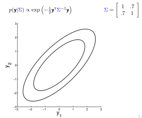
\[ \begin{align} p(\mathbf{y} | \Sigma ) \approx \exp (-\frac{1}{2} \mathbf{y}^T \Sigma \mathbf{y}) \end{align} \]

\[ \Sigma (x_1, x_2) = K(x_1, x_2) + I \sigma_y^2 \]

The covariance matrices in all the above examples are computed using the Radial Basis Function (RBF) kernel and \(\sigma_y\) can be noise term.

Here is an example of a 2D Gaussian distribution with mean 0, with the oval contours denoting points of constant probability.
we can now visualize the sampling operation in a new way by taking multiple "random points"
For conditioning, we can simply fix one of the endpoint on the index graph (in below plots, fix y1 to 1) and sample from y2

Here is an example of a 2D Gaussian distribution with mean 0, with the oval contours denoting points of constant probability.

we can now visualize the sampling operation in a new way by taking multiple "random points"

For conditioning, we can simply fix one of the endpoint on the index graph (in below plots, fix y1 to 1) and sample from y2

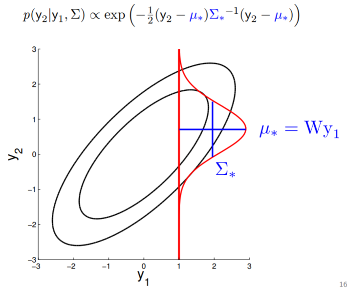
Conditional probability is,

\[ \begin{align} P(A|B) = \frac{P(A \cap B)}{P(B)} \end{align} \tag{1} \]

Get real number

It feels like all the points on the x-axis have to be integers because they are indices, while in reality, we want to model observations with real values.

We can calculate this covariance matrix for any real-valued \(x_1\) and \(x_2\) by simply plugging them in. The real-valued x's effectively result in an infinite-dimensional Gaussian defined by the covariance matrix.