ML | DeepONet
DeepONet
DeepONet is a novel deep learning architecture designed to approximate nonlinear operators, which are mappings from one function space to another. Developed by researchers at Brown University, DeepONet represents a significant advancement in the field of machine learning, particularly in its ability to handle complex mathematical operations typically associated with differential equations.
Architecture
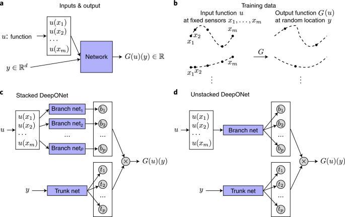
The DeepONet framework consists of two main components:
- Branch Network: This network encodes the input function space, capturing data from discrete sensor locations.
- Trunk Network: This network encodes the output function space, determining how the input data is transformed into outputs.
Together, these networks enable DeepONet to learn a mapping between functions rather than just pointwise values, which is a common limitation of traditional neural networks.
Key Features
- Universal Approximation: DeepONet is grounded in the universal approximation theorem for operators, allowing it to approximate any continuous nonlinear operator with high accuracy. This capability extends beyond what standard neural networks can achieve.
- Speed and Efficiency: Once trained, DeepONet can perform real-time predictions significantly faster than conventional solvers used for differential equations. It can handle complex systems and make predictions in fractions of a second, which is particularly useful in applications like autonomous vehicles and digital twins for real-time modeling.
- Versatility: The architecture can be applied across various domains, including climate modeling, robotics, and even nuclear energy systems. Its ability to generalize from training data allows it to predict outcomes for new inputs that were not part of the training set.
Applications
DeepONet has promising applications in:
- Autonomous Vehicles: Real-time predictions can enhance decision-making processes.
- Digital Twins: It enables accurate modeling of physical systems without the need for extensive retraining under varying conditions.
- Complex Systems Simulation: The architecture can represent intricate behaviors in dynamic environments, making it suitable for tasks such as climate modeling and engineering design.
Universal Approximation Theorem
Definition
The theorem states that for any continuous function $ f: ^n $ defined on a compact subset of $ ^n $, there exists a neural network $ g $ such that the difference between $ f $ and $ g $ can be made arbitrarily small. Formally, for any $ > 0 $, there exists a neural network with a finite number of neurons such that:
\[ | f(x) - g(x) | < \epsilon \]
for all $ x $ in the domain of interest.
Historical Background
The theorem was independently proven by George Cybenko in 1989, who focused on networks using sigmoid activation functions, and later by Kurt Hornik in 1991, who generalized it to include other activation functions like ReLU (Rectified Linear Unit).
Implications
It has profound implications for the design and understanding of neural networks:
- Expressive Power: It guarantees that neural networks can model complex relationships in data, making them suitable for tasks like image classification, function approximation, and more.
- Architecture Design: The theorem informs users about the necessary architecture (e.g., number of layers and neurons) required to achieve desired approximations.
Limitations
While the UAT provides a theoretical foundation, it does not address practical aspects such as:
- Generalization: The ability of a network to perform well on unseen data is not guaranteed by the theorem alone. Techniques like regularization and cross-validation are necessary to improve generalization.
- Computational Feasibility: The theorem does not specify how to construct the network or find the optimal parameters effectively. In practice, training methods like backpropagation are used, but they may not always reach the global optimum.
Reading
Maths
Theorem 5: Suppose that \(g\in (TW)\), \(X\) is a Banach Space, \(K_1 X, K_2 R^n\) are two compact sets in \(X\) and \(R^n\) respectively, \(V\) is a compace set in \(C(K_1)\), \(G\) is a nonlinear continuous operator, which maps \(V\) into \(C(K_2)\), then for any $>0 $, there are positive integers \(M, N, m\) constants \(c_i^k, \zeta_k, \xi_{ij}^k \in R^n\), \(x_j \in K_1, i=1,...,M, k=1,...,N, j=1,...,m\), such that
\[ \begin{align*} | G(u)(y) - \sum_{k=1}^N \sum_{i=1}^M c_i^k g( \sum_{j=1}^m \xi_{ij}^k u(x_{j}) + \theta_i^k) g(\omega_k \cdot y + \xi_k)| < \epsilon, \qquad \forall u \in U \end{align*} \]
More details,
\[ \begin{align*} G(u)(y) &= G(u) \otimes (y) \\ &= \sum_{k=1}^p b_k t_k \\ &= \sum_{k=1}^p b_k \sigma(w_k \cdot y + \zeta_k) \\ &= \sum_{k=1}^p \sum_{i=1}^n c_i^k \sigma(\sum_{j=1}^m \xi_{ij}^k u(x_j) + \theta_i^k) \sigma(w_k \cdot y + \zeta_k) \\ \end{align*} \]
For a trunk net,
\[ \begin{align*} t_k &= \sigma(w_k \cdot y + \zeta_k) \in \mathbb{R} \\ \{t_k\}_{k=1,...,p} &= \{\sigma(w_k \cdot y + \zeta_k)\} \in \mathbb{R}^p \\ \end{align*} \]
For one branch net (num of neuron = \(n\)) , all coefficients are dependent on \(k\),
\[ \begin{align*} b_k = \sum_{i=1}^n c_i^k \sigma(\sum_{j=1}^m \xi_{ij}^k u(x_j) + \theta_i^k) \in \mathbb{R} \end{align*} \]