Pseudo-Global Warming (PGW) - Future Projection
Pseudo-Global Warming (PGW)
Definition and Concept
Pseudo-Global Warming (PGW) is a regional climate modeling approach that involves imposing large-scale climate changes derived from global climate models (GCMs) onto a control regional climate simulation. This method contrasts with traditional dynamic downscaling, where regional models are driven directly by GCM outputs. Instead, PGW modifies the boundary conditions of a historical simulation to reflect projected future changes, allowing for a more flexible and computationally efficient analysis of climate impacts.

To perform future projections using the Pseudo-Global Warming (PGW) approach, follow these key steps:
Methodology for PGW Projections
1. Understanding PGW Concept
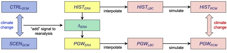
The PGW method involves modifying historical climate simulations by imposing future climate changes directly onto them. This is achieved by adjusting the boundary conditions of a control simulation based on projected changes derived from global climate models (GCMs).
2. Mathematical Representation
The PGW approach can be mathematically expressed as:
\[ \text{PGW} = \text{HIST} + \Delta \]
where:
- HIST represents the current or historical climate conditions.
- Δ (Delta) is the perturbation derived from future climate projections,
calculated as:
\[ \Delta = \text{SCEN} - \text{CTRL} \]
Here, SCEN is a future climate scenario, and CTRL is the corresponding historical baseline.
Both SCEN and HIST periods must be chosen to be long enough to reduce the effects of internal variability (average of ∼ 30 years).
- Chow, T. N., Tam, C. Y., Chen, J., & Hu, C. (2024). Effects of Background Synoptic Environment in Controlling South China Sea Tropical Cyclone Intensity and Size Changes in Pseudo–Global Warming Experiments. Journal of Climate, 37(5), 1811-1832.
- Zhao, R., Tam, C. Y., Lee, S. M., & Chen, J. (2024). Attributing extreme precipitation characteristics in South China Pearl River Delta region to anthropogenic influences based on pseudo global warming. Earth and Space Science, 11(3), e2023EA003266.
- In the second PGW experiment, human‐induced perturbations are computed as the monthly averages of the 30‐year (1986–2005) mean differences between historical and historicalNat runs of CMIP5 seven‐model ensemblemean.
- The perturbed fields include SST, air temperature, specific humidity, and horizontal wind components.
- Brogli, R., Heim, C., Mensch, J., Sørland, S. L., & Schär, C. (2023). The pseudo-global-warming (PGW) approach: methodology, software package PGW4ERA5 v1. 1, validation, and sensitivity analyses. Geoscientific Model Development, 16(3), 907-926.
- Both SCEN and HIST periods must be chosen to be long enough to reduce the effects of internal variability (average of ∼ 30 years).
- After applying Δ to the thermodynamic variables, it is thus essential to restore this balance using an adequate pressure adjustment
- Pseudo Global Warming: Methodology
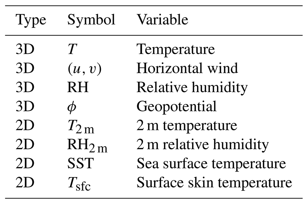
- The perturbation fields Delta are meant to be based on 30-year monthly means of the driving GCM. The required GCM fields include three-dimensional fields of temperature, specific humidity and wind (T, qv, u, v), as well as the geopotential height field (phi) on at least one pressure level. Monthly mean changes of these fields are linearly interpolated to the target date, and then merged with ERA5 information.
3. Data Requirements
To implement PGW, you need:
- Historical climate data (e.g., from reanalysis datasets like ERA5).
- Future climate projections from GCMs, typically focusing on thermodynamic and dynamic variables such as temperature, humidity, wind, and geopotential height.
4. Simulation Setup
- Select a GCM: Choose a transient GCM that provides future climate scenarios relevant to your region of interest.
- Derive Δ: Compute the perturbations (Δ) based on 30-year monthly means from the GCM outputs.
- Modify Boundary Conditions: Apply Δ to the historical data to create new boundary conditions for your regional climate model (RCM) simulations.
5. Running Simulations
- Execute the RCM with the modified boundary conditions. The PGW approach allows for shorter simulation periods (less than 30 years), which can be beneficial for high-resolution climate projections.
- Ensure that interannual variability is not included in these projections since PGW assumes a consistent seasonal cycle.
6. Analyzing Results
After running the simulations:
- Assess changes in key climate variables such as temperature, precipitation, and extreme weather events.
- Compare results with traditional dynamic downscaling methods to validate the PGW approach's effectiveness in capturing plausible future scenarios.
Advantages of PGW
- Computational Efficiency: PGW requires less computational power compared to traditional methods, making it suitable for high-resolution studies.
- Flexibility: It allows researchers to easily modify simulation parameters and assess various future scenarios.
Challenges and Considerations
Despite its advantages, implementing PGW poses challenges:
- Complexity of Implementation: Care must be taken to ensure that modifications do not compromise the physical realism of the regional model. Adjustments to pressure and geopotential fields are critical for maintaining consistency between thermodynamic and dynamic changes.
- Interannual Variability: The PGW method typically does not account for changes in interannual variability, which can limit its applicability in certain contexts.
- Sensitivity to Initial Conditions: The effectiveness of PGW simulations can be sensitive to the choice of initial conditions and boundary settings, necessitating careful calibration.
By following this structured methodology, researchers can effectively utilize the PGW approach to project future climate conditions while addressing specific regional impacts of global warming.
Example
2024 | Zhao & Francis Tam | PRD
Experiment Setup,
- WRF model v3.8.1 (Skamarock et al., 2008) in a one-way nesting setup
- 50 km × 50 km, covering most of southeast Asia, 10 km × 10 km (136 × 116 grid cells) and 2 km × 2 km (181 × 166 grid cells), respectively. There are 45 vertical layers from the surface up to 50 hPa, with 18 layers in the lowest 1.5 km, to resolve the planetary boundary layer (PBL) dynamics.
- Spectral nudging is applied to zonal and meridional wind components above 500 hPa over the outermost domain (Liu et al., 2012; Ma et al., 2016), at the scale of about 1,300 km (1,500 km) in the zonal (meridional) direction.
- 2 Experiments
- In the first set of experiments, or the control (CTL) run, the initial and boundary conditions (IBCs) are taken from ERA-Interim reanalysis
- in the second set of experiments (denoted as the NAT run), the model is forced by the counterfactual IBCs with human-induced climatic perturbations being absent, following the pseudo global warming (PGW) method
- In the second PGW experiment, human-induced perturbations are computed as the monthly averages of the 30-year (1986–2005) mean differences between historical and historicalNat runs of CMIP5 seven-model ensemble mean.
- The perturbed fields include SST, air temperature, specific humidity, and horizontal wind components (Figure S4 in Supporting Information S1).
- The use of a multi-model ensemble mean can minimize the model uncertainty and internal climate variability from the CMIP5 individual models (Liu et al., 2017).
- We define a ratio of observations to seven-model ensemble-mean projections of ST trends as the scale factor that is multiplied by the ensemble-mean perturbations, to resolve more realistic anthropogenic perturbations. ?
- Finally, these perturbations were interpolated linearly on each model grid over the outermost domain and then subtracted from ERA-Interim to generate counterfactual IBCs in WRF.
- This method allows one to estimate anthropogenic influences on a specific extreme event, which makes it easier to perform event attribution analysis based on dynamical downscaling
2022 | Chow | CUHK ESSC M.Phil. thesis
- Tsun Ngai CHOW
- M.Phil. thesis: Effects of Background Synoptic Environment in Controlling the Tropical Cyclone Intensity and Size Changes in South China Sea in Pseudo-Global Warming Experiments
- https://atmosphericdynamicsgroup.github.io/publications.html
- https://atmosphericdynamicsgroup.github.io/theses/Tsun%20Ngai%20CHOW.pdf#page=48.40
- Chow, T. N., Tam, C. Y., Chen, J., & Hu, C. (2024). Effects of background synoptic environment in controlling South China Sea tropical cyclone intensity and size changes in pseudo–global warming experiments. Journal of Climate, 37(5), 1811-1832.
Experiment Setup,

- total of 31 and 5 models from the CMIP5 were selected to obtain the projected future changes following the RCP8.5 and RCP4.5 emission scenario respectively.
- The climate conditions in the 1975 – 1999 were selected as the reference of the historical climate while the climate conditions in the 2036 – 2065 and 2075 – 2099 were selected as the near future and the far future climate respectively.
- The SST, land surface temperature, atmospheric temperature and the specific humidity profiles in the historical climate, as well as in the projected near future and the far future climate were averaged across that period for each month separately to obtain the mean monthly climatic condition in the historical, near future and far future period.
- After that, the SST, land surface temperature, atmospheric temperature and specific humidity in the near future and the far future were subtracted by the historical climate conditions, obtaining the change of surface temperature, atmospheric temperature and the specific humidity profile in the near and the far future relative to the historical period.
- Then, the change in the monthly mean SST, land surface temperature, atmospheric temperature profile and the specific humidity profile in the near future and the far future relative to the historical climate were superimposed on the historical environment of the 25 selected TCs according to the month of occurrence in the past for each TC to create a total of 4 warming experiments, each contain 25 TC cases. Therefore, there are 1 control simulation and 4 warming experiments for each of the 25 TC cases, and a total of 125 simulations.
- Moreover, the reason for not imposing the projected change in wind field in the future climate to the TCs were to examine the change in thermodynamical environment due to global warming to the intensity and the size of the TCs, while not changing the track of the TC. The author aimed to reduce the complexity brought by the possible changes of the TC track in the future environment due to a change of steering wind, which then allowed a comparison between the response of different TCs in a warmed climate by attributing the different in the percentage change of TC intensity and size to the difference in the historical environment and the imposed warming signal.
- WRF-ARW version 3.7, ERA-20C and EAR5 as the initial and boundary conditions of the control run
- 2 nested domains were set up with one-way nesting, with 15 km and 3 km (the domain size is 339 × 249 and 400 × 580 grid), 45 eta levels across the vertical direction
2018 | Gutmann | Changes in hurricanes ...
Experiment Setup,
- The future simulations were forced with the same input data after adding a climate change signal to the data using the pseudo–global warming (PGW) method.
- In these simulations we applied a PGW change for the following input variables: zonal and meridional wind speed, sea level pressure, geopotential height, air temperature, relative humidity, and sea surface temperature as well as initial soil temperatures and the bottom boundary condition in the soil.
- We compute the change signal over a 95-yr time period using data from the representative concentration pathway 8.5 (RCP8.5) scenario for 19 models in the CMIP5 archive. This is calculated by averaging the period 2070–99 and subtracting from it the average over the period 1976–2005. This change signal is calculated independently for every variable at every grid point in space, and for every month of the year.
- Changes are temporally interpolated between month midpoints. For example, the change signal for 15 May of all years is computing by averaging the change signal over the period 1–30 May. The resulting change signal has a mean warming signal of 3–6 deg C and an increase in water vapor mixing ratio of 20%–40%, consistent with the Clausius–Clapeyron relationship.
2011 | Rasmussen
Experiment Setup,
- The PGW methodology consists of adding a climate perturbation signal to a contemporary high-resolution analysis of the atmosphere during the future period of interest. (provides a first-order estimate of the potential climate warming impacts)
- The climate perturbation’s primary impact is on the large-scale planetary waves and associated thermodynamics, while the weather patterns entering the domain boundary remain structurally identical in both simulations in terms of frequency and intensity. The weather events, however, can evolve within the regional model domain due to the altered planetary flow and thermodynamics.
- The monthly climatology’s are the decadal monthly averages for the future and current decades resulting in regional values of mean temperature, vapor mixing ratio, geopotential height, and wind at each vertical level in the model in the domain of the high-resolution simulations.
- The climate perturbation field is added to the current weather field for the selected years by linearly interpolating from the monthly climatologies to each time period in the NARR analysis assuming that the monthly mean is valid on the 16th of the month.
- At the surface, deep-soil temperatures are also perturbed with the same methodology.
- Both the initial conditions and time-evolving lateral and lower boundary conditions from NARR are therefore perturbed with the climate change signal.
- The significant benefit of this is that the climate perturbation signal can be added to the NARR analysis while maintaining hydrostatic and geostrophic balances because the difference of two balanced mean fields retains the linear relationships between the virtual temperature, geopotential height, and horizontal wind perturbation fields. Therefore, adding this difference retains the consistency in the large-scale fields, while also preserving the small-scale weather patterns and imbalances of the period of interest.
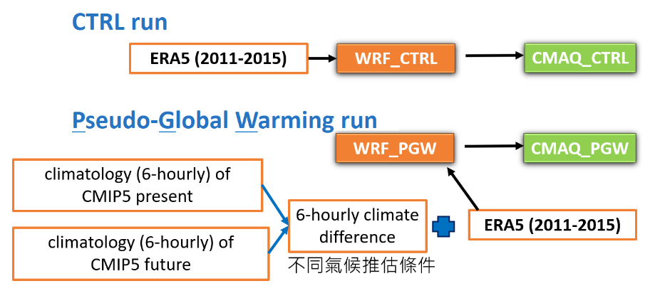
臺灣空氣品質變化與氣候變遷
- 臺灣空氣品質變化與氣候變遷 計畫流程示意圖。預計將進行對照組(CTRL)及實驗組(Pseudo-Global Warming, PGW),分別以WRF及CMAQ模擬現在及未來氣候狀態的空氣品質。橘色框為WRF初始及邊界條件,CTRL使用ECMWF ERA5資料,PGW則考慮未來氣候變化差異。
Code/Software
** Software package PGW4ERA5 v1.1
- Brogli, R., Heim, C., Mensch, J., Sørland, S. L., & Schär, C. (2023). The pseudo-global-warming (PGW) approach: methodology, software package PGW4ERA5 v1. 1, validation, and sensitivity analyses. Geoscientific Model Development, 16(3), 907-926.
- The term “pseudo-global warming” (PGW) refers to a simulation strategy in regional climate modeling. The strategy consists of directly imposing large-scale changes in the climate system on a control regional climate simulation (usually representing current conditions) by modifying the boundary conditions.
- Both SCEN and HIST periods must be chosen to be long enough to reduce the effects of internal variability (average of ∼ 30 years).
- At first glance it is surprising that one can change the driving fields of an RCM simulation in an ad hoc fashion as depicted above without introducing serious inconsistencies in the atmospheric dynamics. ... However, the PGW approach rests on a solid theoretical foundation....In essence, the balanceof forces is unchanged...
As to be demonstrated later (see Sect. 4.3), it is advantageous to use relative humidity (RH) rather than qv; if only the latter is available, qv is converted into RH. There are alternative approaches to treat the humidity change, such as the assumption of no change in RH with warming
CMIP5_to_WRF
Bias-corrected GCMs/CMIP6 Global dataset
Calibration and bias correction


- Eqn. A.2 is a mapping \(f: X_1 \mapsto X_2\) with providing estimates of \(M_{1,2}\) and \(\sigma_{1,2}\).
- then, we can map any input and get corresponding f(input) with providing estimates of \(M_{1,2}\) and \(\sigma_{1,2}\).
- like $ T_{BC} (t) = f(T_{RAW}(t))$ with providing estimates of \(M_{1,2}\) and \(\sigma_{1,2}\).
An Evaluation of Statistical and Dynamical Techniques for Downscaling Local Climate

建立環流模式推估能力評比之方法
- 連宛渝, 童慶斌, 何宜昕, 戴嘉慧, & 莊立昕. (2013). 建立環流模式推估能力評比之方法. 農業工程學報, 59(1), 1-14.
- GCM 模擬結果與地面測站資料存在著誤差,在進行簡易降尺度之前,必須藉由誤差修正(Bias Correction)才能去除模式與地面測站之間的系統誤差。
- 假設GCM 之輸出資料. 與地面測站資料有相同之統計特性,亦即具有相. 同之機率值的情況下,GCM 之逐月資料與歷史. 逐月資料之關係可由式(1)表示
- By \(pdf = \frac{1}{\sqrt{2\pi\sigma^2}} e^{-\frac{(x - \mu)^2}{2\sigma^2}}\)
- \(\frac{X_{obs} - \mu_{obs}}{\sigma_{obs}} = \frac{X_{GCM} - \mu_{GCM}}{\sigma_{GCM}}\)
Bias-corrected CMIP6 global dataset for dynamical downscaling of the historical and future climate (1979–2100)
- Xu, Z., Han, Y., Tam, C. Y., Yang, Z. L., & Fu, C. (2021). Bias-corrected CMIP6 global dataset for dynamical downscaling of the historical and future climate (1979–2100). Scientific Data, 8(1), 293.
- General Circulation Model (GCM) is/are known to have significant biases, which propagate into RCMs through the lateral boundary and thus degrade the downscaled simulations.
- We constructed a bias-corrected global dataset based on 18 models from the Coupled Model Intercomparison Project Phase 6 (CMIP6) and the European Centre for Medium-Range Weather Forecasts Reanalysis 5 (ERA5) dataset.
- The bias-corrected data have an ERA5-based mean climate and interannual variance, but with a non-linear trend from the ensemble mean of the 18 CMIP6 models.
- The dataset spans the historical time period 1979–2014 and future scenarios (SSP245 and SSP585) for 2015–2100 with a horizontal grid spacing of (1.25° × 1.25°) at six-hourly intervals.
- However, GCMs are known to have significant biases, which propagate into RCMs through the lateral boundary and thus degrade the downscaled simulations
- Our method takes advantage of the non-linear trend of the ensemble mean of 18 Coupled Model Intercomparison Project Phase 6 (CMIP6) models to give a more reliable projection of the long-term climate trend.
- In addition, we also correct the GCM climatological mean and interannual variance biases based on the European Centre for Medium-Range Weather Forecasts Reanalysis 5 (ERA5) dataset.


基于 CMIP6 耦合 WRF 的黄河上游复合干旱热浪事件演变规律. 水利学报, 55(8), 908-919.
- 门宝辉, 吕行, 陈仕豪, & 王红瑞. (2024). 基于 CMIP6 耦合 WRF 的黄河上游复合干旱热浪事件演变规律. 水利学报, 55(8), 908-919.
- http://jhe.ches.org.cn/jhe/ch/reader/create_pdf.aspx?file_no=20240803&flag=1&journal_id=jhe&year_id=2024#page=1.00&gsr=0
- 本文提出了一种基于第六次国际耦合模式比较计划CMIP6耦合天气预报研究模式WRF的未来气象数据动力降尺度方法
- 精度验证
- 采用研究区域内10个气象站(如图1所示)1979-2014年的实测数据及5种原始CMIP6数据集对bc-CMIP6的模拟精度进行检验和对比

