Climate models

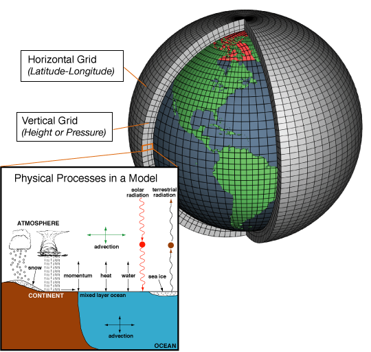
Climate models are systems of differential equations based on the basic laws of physics, fluid motion, and chemistry. To "run" a model, scientists divide the planet into a 3-dimensional grid, apply the basic equations, and evaluate the results. Atmospheric models calculate winds, heat transfer, radiation, relative humidity, and surface hydrology within each grid and evaluate interactions with neighboring points.

(Image source: NOAA)

The complexity of the climate models

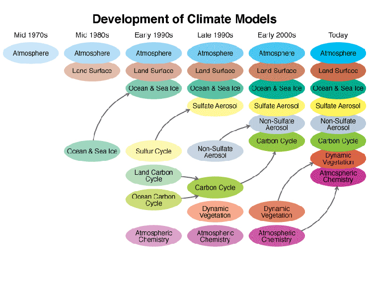
As computing power has increased since the 1970s, so has the complexity of the computer models used to simulate Earth's climate. Components are first developed separately and later coupled into comprehensive models.

(From NASA)

Climate model bias

Climate model bias is the difference between the statistics of the observations for the reference period and the statistics of the climate model simulation for the same period.

The bias of a climate model is determined by comparing the climate model output for a past period with observational data for that same period. For example the annual and seasonal climatological averages for all relevant climate variables are compared, the probability of certain extremes, variability, trends, etc. The smaller the bias, the higher the model skill to simulate the observed climate correctly. This skill is often used as a measure of quality. Model biases are determined by comparing the statistics of observational records for a certain period (often 30 years) with the simulated climate for the same period in the past (for projections). Biases can not be determined by comparing e.g. the weather on certain dates or in certain years in the past!

• Gupta, A. S., Jourdain, N. C., Brown, J. N., & Monselesan, D. (2013). Climate Drift in the CMIP5 Models. Journal of Climate, 26(21), 8597-8615. https://doi.org/10.1175/JCLI-D-12-00521.1
  • Model drift refers to spurious long-term changes in general circulation models that are unrelated to either changes in external forcing or internal low-frequency variability. Drift can be caused by a number of factors. For example, a simulation's initial state may not be in dynamical balance with the representation of physics in the model; “coupling shock” may occur during the coupling of model components resulting in discontinuities in surface fluxes (e.g., Rahmstorf 1995) or numerical errors may exist in the model that mean that heat or moisture is not fully conserved

Climate model bias refers to the systematic differences between the outputs of climate models and actual observed climate statistics. These biases can arise from several factors, including:

1. Definition of Climate Model Bias

• Climate model bias is defined as the difference between a simulated climate statistic (from a model) and the corresponding real-world climate statistic (observations) for the same period. This can include discrepancies in temperature, precipitation, and other climate variables over time.

2. Causes of Bias

• Spatial Resolution: Many climate models operate on large grid sizes, which can lead to inaccuracies in representing local climate features.
• Simplified Thermodynamic Processes and Physics: Models may oversimplify complex physical processes, such as convection or land-atmosphere interactions, leading to incorrect simulations of climate dynamics.
• Incomplete Understanding: The current understanding of the climate system is not exhaustive, which can result in biases in model outputs.

3. Types of Bias

• Mean Bias: The average difference between model outputs and observations.
• Variance Bias: Differences in variability, such as how extreme weather events are represented.
• Temporal Bias: Issues related to timing, such as incorrect seasonal patterns or shifts in monsoon timings.

4. Implications of Bias

Using uncorrected climate model outputs for impact assessments can yield unrealistic results. For example, if a model consistently underestimates rainfall extremes, it could misinform water resource management or flood risk assessments.

5. Bias Correction Methods

To address these biases, various statistical methods have been developed:

• Delta Change Method:
  • Adjusts historical observations based on projected changes from models (e.g., adding a predicted temperature increase to historical data).
  • The simplest approach is the Delta change method, which is often used in climate impact research. This approach uses the GCM or RCM response to climate change to modify observations. E.g. if the climate model predicts 3°C higher temperatures, 3°C is added to all historic observations to construct a new time series for the future climate. For rainfall usually a percentage change is calculated. If the climate model predicts a 20% increase in rainfall, a new time-series will be made by multiplying the historic rainfall by 1.2. For different months or seasons different delta factors can be defined. Note: this method does not take into account changes in climate variability such as increasing extreme rainfall or longer dry spells.
• Quantile Mapping: A more sophisticated method that maps the cumulative distribution functions (CDFs) of observed and modeled data to adjust for biases across all quantiles.
• Linear Regression: Uses historical data to create a statistical relationship between observed and modeled outputs for future projections.

Both the delta change and linear regression method are suitable to bias adjust relative humidity, humidity, wind speed and radiation.

Climate models produce area-average data, whereas many observations are point measurements. In order to determine the skill, climate model data should be compared with area-average data, otherwise the bias may be affected by the difference between area-average and point data. This is especially important for climate variables where large spatial differences are observed within a grid cell, e.g. precipitation. For this reason reanalysis data are often used to determine the skill of climate models. The quality of climate data for the future cannot be assessed in a direct way, since no observational data set is available for the future. It is generally assumed that the bias/skill for the future is the same as for the past/current climate (although this is not necessarily true). When the skill is good for the current climate, we generally have more confidence in the results for the future.

6. Challenges with Bias Correction

While bias correction methods aim to improve model outputs, they have limitations:

• They may not fully correct underlying physical process misrepresentations.
• They can introduce new artifacts or inconsistencies in spatial and temporal data.
• The assumption that present-day biases will remain constant over time can be problematic, especially for variables like precipitation that may exhibit non-stationarity.

In summary, understanding and correcting climate model bias is essential for improving the reliability of climate projections and their applications in impact studies.

Downscaling climate models

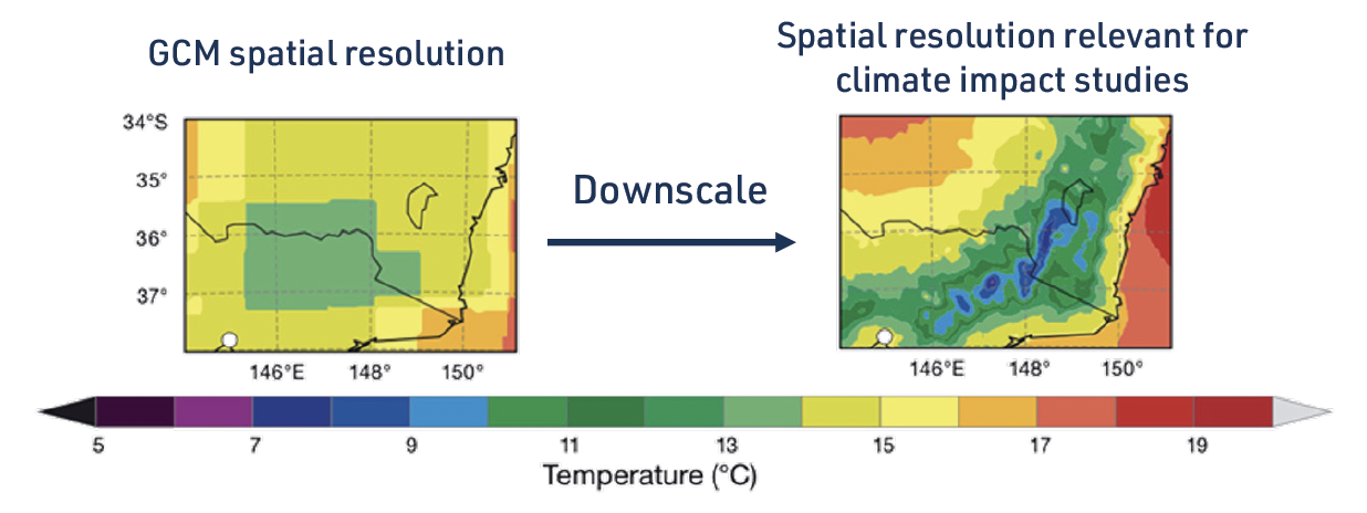
Downscaling climate models is a crucial process for obtaining localized climate information from global climate models (GCMs), which typically operate at coarse spatial resolutions. Below is an overview of how to perform downscaling and the associated challenges.

Downscaled temperature over south-east Australia. Data: NARCLiM

• 什麼是降尺度? 為什麼降尺度不是越細越好?

Methods of Downscaling

1. Types of Downscaling

• Dynamical Downscaling: This method uses regional climate models (RCMs) that are forced by GCM outputs. RCMs operate on finer spatial scales (typically <50 km) and can capture local climate features more accurately by incorporating detailed physical processes.
• Statistical Downscaling: This approach establishes statistical relationships between large-scale climate variables from GCMs and local observations. It is less computationally intensive than dynamical downscaling and includes methods such as:
  • Bias Correction with Spatial Disaggregation (BCSD): Adjusts GCM outputs based on historical data.
  • Quantile Mapping: Corrects the distribution of model outputs to match observed data distributions.
  • Localized Constructed Analogs (LOCA): Finds analogous historical weather patterns to generate fine-resolution outputs.

2. Steps for Downscaling

1. Select a GCM: Choose a suitable global climate model and the relevant emission scenario.
2. Obtain Historical Data: Gather historical climate data for the region of interest to establish baseline conditions.
3. Choose a Downscaling Method: Decide between dynamical or statistical downscaling based on available resources and required precision.
4. Run the Downscaling Model:
   • For dynamical downscaling, set up the RCM with appropriate boundary conditions from the GCM.
   • For statistical downscaling, develop statistical relationships using historical data and apply them to future GCM projections.
5. Validate Outputs: Compare downscaled results with observed data to assess accuracy and make necessary adjustments.

Challenges of Downscaling

1. Computational Demands

• Both dynamical and statistical downscaling can be computationally intensive, especially when multiple RCMs or scenarios are involved. This can strain resources for many research groups, limiting their ability to conduct extensive simulations.

2. Bias Issues

• GCMs often have systematic biases in their outputs, which can propagate through the downscaling process. If not adequately addressed, these biases can lead to misleading local projections.

3. Uncertainty in Atmospheric Circulation

• The accuracy of downscaled projections is heavily reliant on the atmospheric circulation patterns provided by GCMs. Any uncertainty in these patterns can significantly affect regional climate outcomes.

4. Limitations of Statistical Methods

• Statistical downscaling relies on historical relationships that may not hold true under future climate conditions, leading to potential inaccuracies in projections. Additionally, assumptions made during statistical modeling can introduce further biases.

5. Scale Mismatch

• The coarse resolution of GCMs may not adequately represent localized phenomena such as orographic precipitation or extreme weather events, which are vital for impact assessments.

In summary, while downscaling is essential for obtaining high-resolution climate information necessary for local impact studies, it comes with significant challenges that need careful consideration and management to ensure reliable projections.

References

• C3S User Learning Services Data Resources - Climate Models ((Recommendation))
• climateextremes.org.au: Types of models ((Recommendation))
• The difference between weather and climate
• Weather and Climate @ Reading: Weather vs. Climate Prediction
• Climate gov: Climate Models
• earth-scan: weather-vs-climate
• Copernicus Climate Change Service – Global Impacts: What is bias correction?
• Kotamarthi R, Hayhoe K, Mearns LO, Wuebbles D, Jacobs J, Jurado J. Empirical-Statistical Downscaling. In: Downscaling Techniques for High-Resolution Climate Projections: From Global Change to Local Impacts. Cambridge University Press; 2021:82-101. (link)
• Xu, Z., Y. Han, C.-Y. Tam, Z.-L. Yang and C. Fu, 2021: A bias-corrected CMIP6 global dataset. for dynamical downscaling of future climate, 1979–2100, Scientific Data, doi: 10.1038/s41597-021-01079-3. https://atmosphericdynamicsgroup.github.io/database/cmip6.html
• Probable Futures 是一项非营利性气候扫盲计划