NWP | Anomaly Correlation Coefficient (ACC)

Anomaly Correlation Coefficient (ACC)

• https://confluence.ecmwf.int/display/FUG/Section+6.2.2+Anomaly+Correlation+Coefficient
• ECMWF_ACC_definition

The Anomaly Correlation Coefficient (ACC) is one of the most widely used measures in the verification of spatial fields. It is the spatial correlation between a forecast anomaly relative to climatology, and a verifying analysis anomaly relative to climatology. ACC is a measure of how well the forecast anomalies have represented the observed anomalies. It shows how well the predicted values from a forecast model "fit" with the real-life data. ACC for a series of forecast lead-times is a measure of how well trends in the predicted anomalies follow trends in actual anomalies.

The correlating forecasts directly with observations or analyses may give misleadingly high values because of the seasonal variations. It is therefore established practice to subtract the climate average from both the forecast and the verification and to verify the forecast and observed anomalies according to the anomaly correlation coefficient (ACC).

ACC values lie between +1 and -1. Where ACC values:

• approach +1 there is good agreement and the forecast anomaly has had value.
• lie around 0 there is poor agreement and the forecast has had no value.
• approach –1 the agreement is in anti-phase and the forecast has been very misleading.

Where the ACC value falls below 0.6 it is considered that the positioning of synoptic scale features ceases to have value for forecasting purposes.

What the ACC Measures

The fundamental purpose of the ACC is to determine how well the forecast model captures the large-scale pattern and location of weather features that deviate from the long-term normal (the climatology).

1. Anomaly Calculation: An anomaly is the deviation of a variable (e.g., \(500 \text{ hPa}\) geopotential height) from its long-term average for that specific time and location (the climatology).
   • Forecast Anomaly (\(F'\)): \(\text{Forecast} - \text{Climatology}\)
   • Observed Anomaly (\(A'\)): \(\text{Observation} - \text{Climatology}\)
2. Correlation: The ACC is the Pearson correlation coefficient applied to the forecast anomalies (\(F'\)) and the observed anomalies (\(A'\)) across all grid points in the verification domain (e.g., the Northern Hemisphere).

The ACC is a measure of the pattern accuracy, not the magnitude of the errors.

The Formula

The ACC is mathematically defined as the spatial correlation between the forecast anomaly and the analysis (observed) anomaly:

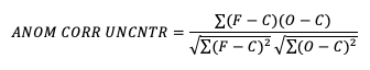
\[ \text{ACC}_\text{uncentered} = \frac{\sum_i w_i F'_i A'_i} {\sqrt{\sum_i w_i (F'_i)^2}\,\sqrt{\sum_i w_i (A'_i)^2}} \]

or

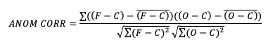
\[\text{ACC}_\text{centered} = \frac{\sum_{i=1}^{N} w_i (F'_i - \overline{F'}) (A'_i - \overline{A'})}{\sqrt{\sum_{i=1}^{N} w_i (F'_i - \overline{F'})^2} \sqrt{\sum_{i=1}^{N} w_i (A'_i - \overline{A'})^2}}\]

Where:

• \(N\) is the total number of grid points in the domain.
• \(F'_i\) is the forecast anomaly at grid point \(i\).
• \(A'_i\) is the observed anomaly at grid point \(i\).
• \(\overline{F'}\) and \(\overline{A'}\) are the spatial mean of the forecast and observed anomalies, respectively (often calculated using weighting).
• \(w_i\) is the area weighting coefficient for grid point \(i\) (used because grid cells closer to the poles cover a smaller area).
  • To counteract the shrinking area of grid cells towards the poles, the most common and standard way to calculate the area weighting coefficient is using the cosine of the latitude (\(\phi_i\)) for each grid point \(i\):
    • \[\mathbf{w_i \propto \cos(\phi_i)}\]
      • At the Equator (\(\phi = 0^{\circ}\)): \(\cos(0^{\circ}) = 1\). The weighting is maximum, as these grid cells cover the largest area.
      • Near the Poles (\(\phi \approx 90^{\circ}\)): \(\cos(90^{\circ}) \approx 0\). The weighting is near zero, effectively down-weighting the small grid cells to ensure they don't overly influence the final result.
    • By multiplying the forecast and observed anomalies by \(\cos(\phi_i)\) before summing them in the numerator and denominator of the ACC formula, the calculation is essentially performed over an equal-area basis.
    • In practice, the ACC formula uses the weighted sum of anomalies and their squares, ensuring the final correlation value accurately reflects the skill of the forecast model across the entire geographical domain.

The ACC ranges from -1 to +1, similar to the standard correlation coefficient:

ACC Value	Interpretation	Skill Implication
+1.0	Perfect correlation. The forecast and observed anomaly patterns are identical.	Perfect Skill
+0.6	Typically considered the threshold where the forecast retains useful synoptic skill (good enough for general weather prediction).	Useful Skill
0.0	No correlation. The forecast pattern is no better than a random pattern.	No Skill
-1.0	Perfect negative correlation. The forecast pattern is completely opposite of the observed pattern.	Very Misleading Forecast

Key Applications

• Medium-Range Forecasts: The ACC of the \(500 \text{ hPa}\) geopotential height (a proxy for the jet stream and large weather systems) is often the headline score used by major weather centers like ECMWF to track skill improvement over time.
• Forecast Horizon: ACC is commonly plotted against forecast lead-time (days) to determine the effective limit of predictability. For instance, if the ACC drops to \(0.6\) at Day 10, the forecast is considered useful up to 10 days.

ACC vs. Other Metrics

The ACC is excellent for pattern but has limitations:

Metric	Focus	Sensitivity
ACC	Pattern and Phase (Are the highs and lows in the right place?)	Not sensitive to bias (the difference in the mean magnitude). A forecast that is too cold everywhere but has the correct pattern will still score high.
Root Mean Square Error (RMSE)	Magnitude of error (How far off are the values in standard units?)	Sensitive to both pattern error and overall forecast bias.

Uncentered vs. centered

1. Verification Statistics for Continuous Forecasts | dtcenter
   1. Anomaly Correlation
   2. There are two widely used versions of anomaly correlation.
      1. The first is the centered anomaly correlation, which includes the mean error relative to the climatology. This version is calculated using
      2. 
      3. If it is not desirable to include the errors, the uncentered anomaly correlation is the better choice:
      4. 

Anomaly correlation coefficient (ACC) can be defined in two slightly different ways, often called centered and uncentered; the distinction is about whether you remove the sample mean of the anomalies themselves before computing the correlation.

Uncentered anomaly correlation

The Uncentered ACC is a less common variation that measures the correspondence between the two anomaly fields without removing their spatial means.

This is what operational NWP centers almost always mean by “ACC”:

• Define anomalies relative to a climatology \(C\): \[ F'_i = F_i - C_i,\quad A'_i = A_i - C_i \]
• Compute the correlation directly from these anomalies, without removing any additional mean: \[ \text{ACC}_\text{uncentered} = \frac{\sum_i w_i F'_i A'_i} {\sqrt{\sum_i w_i (F'_i)^2}\,\sqrt{\sum_i w_i (A'_i)^2}} \]

Here the only centering is the subtraction of climatology; there is no subtraction of the domain/sample mean of \(F'\) or \(A'\).

This version keeps information about systematic errors relative to climatology (mean forecast anomaly vs. mean observed anomaly over the domain).

Key Features:

• No Removal of Spatial Mean: The spatial averages (\(\overline{F'}\) and \(\overline{A'}\)) are not subtracted.
• Sensitive to Bias: The \(\text{ACC}_{\text{uncentered}}\) score is penalized if the overall spatial mean of the forecast anomaly differs significantly from the observed spatial mean anomaly. Therefore, it is sensitive to the overall bias of the forecast's anomaly field.
• Focus: It evaluates the pattern match and the similarity in the average magnitude of the anomalies across the domain.

Centered anomaly correlation

The Centered ACC is the standard and most commonly used form in meteorological and climate forecast verification. It is calculated by first removing the spatial mean from both the forecast anomaly field (\(F'\)) and the observed anomaly field (\(A'\)).

The centered ACC is the Pearson product-moment correlation coefficient of the two anomaly fields:

\[\text{ACC}_{\text{centered}} = \frac{\sum w_i (F'_i - \overline{F'}) (A'_i - \overline{A'})}{\sqrt{\sum w_i (F'_i - \overline{F'})^2} \sqrt{\sum w_i (A'_i - \overline{A'})^2}}\]

Where \(F'_i\) is the forecast anomaly, \(A'_i\) is the observed anomaly, \(\overline{F'}\) and \(\overline{A'}\) are the spatial mean anomalies, and \(w_i\) is the area weighting coefficient.

Key Features:

• Removal of Spatial Mean: The spatial average of the anomalies (\(\overline{F'}\) and \(\overline{A'}\)) is subtracted from the respective fields before calculating the correlation.
• Insensitive to Bias: The \(\text{ACC}_{\text{centered}}\) measures the similarity of the two patterns' shapes, regardless of the magnitude difference (bias) between the overall spatial mean of the forecast anomaly and the observed anomaly.
• Focus: It only evaluates the pattern match and phase agreement (i.e., whether the predicted high-pressure systems and low-pressure systems are in the correct geographical locations).

Summary of the Difference

Feature	Centered ACC (\(\text{ACC}_{\text{centered}}\))	Uncentered ACC (\(\text{ACC}_{\text{uncentered}}\))
Calculation	Removes the spatial mean (\(\overline{F'}\) and \(\overline{A'}\)) from the anomaly fields.	Does NOT remove the spatial mean from the anomaly fields.
Sensitivity	Insensitive to the forecast's overall bias.	Sensitive to the forecast's overall bias.

For example, if a model correctly predicts a cold air outbreak over North America but predicts that the air is \(2^\circ \text{C}\) colder on average than what was observed across the domain, the Centered ACC would still be very high (due to the correct pattern), while the Uncentered ACC would be noticeably lower (penalized for the \(2^\circ \text{C}\) cold bias).

ERA5 for Climatological term

1. Defining Climatology (Climate Normal)

• A Climatology (or Climate Normal) is the long-term average of a meteorological variable, typically calculated over a 30-year period (e.g., 1981–2010 or 1991–2020) as defined by the World Meteorological Organization (WMO).
• ERA5's Role: Since ERA5 provides consistent, continuous, gridded data for a long period (1940–present), researchers can use it to calculate climatologies for virtually any location on Earth for which ERA5 has data. For example, the mean temperature for every January 1st over the 1991–2020 period is derived directly from ERA5 data.

2. Calculating Anomalies

• An Anomaly is the deviation of a specific weather event or period from the climatological normal.
• ERA5's Role: By subtracting the long-term climatology (calculated from ERA5) from the hourly or daily ERA5 value for a specific day, you get the anomaly. This is essential for studying extreme events (e.g., a heatwave's temperature anomaly) and for climate monitoring (e.g., global temperature anomalies).

3. Consistency and Homogeneity

• Climatological studies rely on homogeneity—the data must be comparable across the entire time series.
• ERA5's Role: It achieves this by using a single, modern, fixed numerical weather prediction model and data assimilation system to integrate all observations (satellite, ground station, etc.) from the past 80+ years. This process "fills the gaps" where observations were sparse and ensures that changes in the climate signal are due to the atmosphere, not due to changes in the measurement instruments or models over time.

In summary, when a climate scientist mentions a climatological mean, anomaly, or reanalysis in the context of global data, they are most often referring to calculations derived from a product like ERA5.

ERA5 download

• ERA5 hourly data on single levels from 1940 to present
  • https://cds.climate.copernicus.eu/datasets/reanalysis-era5-single-levels?tab=overview
• ERA5 hourly data on pressure levels from 1940 to present
  • https://cds.climate.copernicus.eu/datasets/reanalysis-era5-pressure-levels?tab=overview
• ERA5 monthly averaged data on single levels from 1940 to present
  • https://cds.climate.copernicus.eu/datasets/reanalysis-era5-single-levels-monthly-means?tab=overview
• ERA5 monthly averaged data on pressure levels from 1940 to present
  • https://cds.climate.copernicus.eu/datasets/reanalysis-era5-pressure-levels-monthly-means?tab=download

Downloading ERA5 Single-Layer Data

This guide provides instructions for downloading single-layer atmospheric variables from the ERA5 reanalysis dataset using the ECMWF CDS API (Climate Data Store Application Programming Interface).

Important Data Caveats

1. Daily Updates and Preliminary Data (ERA5T)

• The ERA5 dataset is updated daily with a latency of approximately 5 days.
• The most recent data is initially released as ERA5T (T for "Timely"). This is a preliminary release.
• In the event that serious flaws are detected in the ERA5T data, the final re-release (which occurs 2 to 3 months later) may contain corrections and differ from the ERA5T version. Users are notified if such differences occur.

2. File Format and Size

• All data downloaded via the CDS API is typically provided in GRIB format.
• For bulk data processing or conversion to NetCDF, consider using tools like grib_to_netcdf (with the -k 4 flag for large files) or Python libraries like xarray and cfgrib.

Standard Single-Layer Download

Requests Mean Sea Level Pressure (msl), 2m Temperature (t2m), and 10m wind components (u10, v10) for a single day.

Then,

grib_to_netcdf -k 4 file_6h.grib -o ERA5_single_yyyy_6h.nc"

Downloading ERA5T (Real-Time Data)

If you need the very latest, most current data (the ERA5T version, which is generally available up to 5 days ago)

Pressure Level Data Download

Use a common subset for efficiency:

pressure_levels = [
    '200', '500', '700', '850'
]

Then,

grib_to_netcdf -k 4 file_6h.grib -o ERA5_plevs_yyyy_6h.nc"

Build the ERA5 climatology field

The goal is a mean state (climatology) \(C(t_{\text{cal}}, x)\) for each calendar time and grid point, using only ERA5.

• Decide which ERA5 product to use (hourly, daily or monthly) and which variable, e.g. 500 hPa geopotential height, 850 hPa temperature, 2 m temperature, etc.
• Select a long reference period, typically 30 years such as 1981–2010 or 1991–2020, so the climatology is stable.

1. Extract ERA5 for the full reference period for your variable and pressure level.
2. Decide temporal resolution for climatology:
   • Daily: all 1 Jan values across years, all 2 Jan, … (possibly smooth with a running window).
   • Monthly: all Januaries, all Februaries, etc.
3. For each calendar day (or month) and grid point, average across all years:
   \[ C(d, x) = \frac{1}{N_{\text{years}}} \sum_{y=1}^{N_{\text{years}}} \text{ERA5}(y, d, x) \]
   where \(d\) is the day-of-year (or month) index and \(x\) is the grid point.

This yields a 3‑D array for daily climatology: \((\text{day}, \text{lat}, \text{lon})\), or \((\text{month}, \text{lat}, \text{lon})\) for monthly.

Implementation notes

• For daily climatology, you may use a running window \((± 7 days)\) for smoother anomalies. link
• For climate normals (monthly or annual), use monthly groupings.
• For soil moisture or other surface variables, ERA5-Land provides higher spatial resolution.

Align model forecasts and ERA5 analyses with climatology

• For each forecast valid time \(t\), determine its calendar day (or month) \(d\).
• Interpolate the climatology \(C(d, x)\) in time if needed, e.g. from monthly mean \(C(\text{month}, x)\) to daily valid times.
• Make sure the climatology is defined on the same grid as the forecast and analysis fields; if not, interpolate ERA5 or the model fields to a common grid first.

Compute anomalies

For each forecast case and grid point \(x\):

• Forecast anomaly:
  \[ F'(t, x) = F(t, x) - C(d(t), x) \]
  
• Analysis (verification) anomaly using ERA5:
  \[ A'(t, x) = A(t, x) - C(d(t), x) \]

Using the same climatology for both is essential; do not use separate climatologies for forecast and verification when computing ACC.

Average anomalies over time / cases / domain if desired

Often ACC is computed for a sample of forecasts at the same lead time over many initial dates.

• Collect all \(F'\) and \(A'\) at a given lead time over the selected period.
• Compute spatial means needed for correlation using that full set, e.g. subtract the spatial mean anomaly before computing covariance if using the covariance form of ACC. [be or not be]

This yields one ACC value per lead time (and region and variable).

ERA5: check: convert Gregorian time to datetime

• To check the validation of time of ERA5
• To convert the time value from an ECMWF/ERA5 NetCDF file using Python's datetime and timedelta modules.

▶

convert gregorian time to datetime

import argparse
from datetime import datetime, timedelta

def convert_ecmwf_time(ecmwf_time_value):
    """
    Converts a time value (in hours since the epoch) from ECMWF data 
    to a Gregorian datetime object.
    """
    # Define the epoch as specified in the NetCDF 'time:units' attribute
    # For ECMWF data, this is commonly '1900-01-01 00:00:00.0'
    epoch_date = datetime(1900, 1, 1, 0, 0, 0)

    # Calculate the timedelta from the epoch
    time_delta = timedelta(hours=ecmwf_time_value)

    # Add the timedelta to the epoch to get the Gregorian datetime
    gregorian_datetime = epoch_date + time_delta

    print(f"--- ECMWF Time Conversion ---")
    print(f"Epoch Date: {epoch_date}")
    print(f"Input Time Value: {ecmwf_time_value} hours")
    print(f"Time Delta: {time_delta}")
    print(f"Gregorian Datetime: {gregorian_datetime}")
    print(f"-----------------------------")

if __name__ == "__main__":
    # 1. Create the ArgumentParser object
    parser = argparse.ArgumentParser(
        description="Convert ECMWF time (hours since 1900-01-01) to a Gregorian datetime."
    )

    # 2. Add the argument for the ECMWF time value
    parser.add_argument(
        "ecmwf_time",
        type=int,  # Specify that the input should be an integer
        help="The ECMWF time value in hours (e.g., 1000000)."
    )

    # 3. Parse the arguments from the command line
    args = parser.parse_args()

    # 4. Call the conversion function with the parsed argument
    convert_ecmwf_time(args.ecmwf_time)

grib files: Duplicate

 $ grib_to_netcdf 580de9ac434a7edcacca1626ec12410e.grib -o ERA5_v10_1990_2010.nc
grib_to_netcdf: Version 2.19.1
grib_to_netcdf: Processing input file '580de9ac434a7edcacca1626ec12410e.grib'.
ECCODES ERROR   :  Wrong number of fields
ECCODES ERROR   :  File contains 7698 GRIBs, 7698 left in internal description, 7670 in request
ECCODES ERROR   :  The fields are not considered distinct!
ECCODES ERROR   :  Hint: This may be due to several fields having the same validity time.
ECCODES ERROR   :  Try using the -T option (Do not use time of validity)

$ grib_to_netcdf -T 580de9ac434a7edcacca1626ec12410e.grib -o v10.nc
grib_to_netcdf: Version 2.19.1
grib_to_netcdf: Processing input file '580de9ac434a7edcacca1626ec12410e.grib'.
ECCODES ERROR : Wrong number of fields
ECCODES ERROR : File contains 7698 GRIBs, 7698 left in internal description, 7670 in request
ECCODES ERROR : The fields are not considered distinct!
ECCODES ERROR : Hint: This may be due to several fields having the same date, time and step.

• check duplicated terms

grib_ls 580de9ac434a7edcacca1626ec12410e.grib  > log
sort log | uniq -d

• python script

#!/bin/python
# -*- coding: utf-8 -*-

import xarray as xr

# 1. Define the input and output filenames
input_file = '580de9ac434a7edcacca1626ec12410e.grib'
output_file = 'unique_fields.nc'

print(f"Loading GRIB file: {input_file}...")

# 2. Load the GRIB file into an xarray Dataset
# cfgrib automatically detects the unique dimensions (like time, step, level)
# and combines the fields. This is where the duplicates are handled.
# The 'default' engine is cfgrib.
try:
    ds = xr.open_dataset(
        input_file,
        engine='cfgrib',
        # Set the backend_kwargs to control how cfgrib handles non-distinct fields.
        # This tells cfgrib to aggressively combine fields based on keys.
        #backend_kwargs={'read_keys': ['dataDate']}
    )
    
    print("Successfully loaded the file. Duplicates have been handled.")
    
    # 3. Save the resulting xarray Dataset back to a new GRIB file
    # This will write out only the unique, combined fields.
    ds.to_netcdf(output_file)
    
    print(f"Clean GRIB file saved as: {output_file}")
   
except Exception as e:
    print(f"An unexpected error occurred: {e}")

• check dimensions of .nc filenames

netcdf unique_fields {
dimensions:
	time = 7670 ;
	latitude = 721 ;
	longitude = 1440 ;

# Remark: correct one is
#netcdf ERA5_t2m_1990_2010 {
#dimensions:
#	longitude = 1440 ;
#	latitude = 721 ;
#	time = 7670 ;
#variables:

proleptic_gregorian vs gregorian

Your original time data (1292630400, 1292716800, ...) are large integers, suggesting units of seconds since a distant epoch (likely 1970-01-01).

Your target time data (1060272, 1060296, ...) are much smaller integers, suggesting units of hours (or days) since a more recent epoch.

To make this transformation, you need to use the cdo settime or cdo setreftime functions to redefine the time axis based on a new reference date and time unit.

• cdo setreftime change the format of time units
• Change the format of time:units
• New time format in ERA5 netcdf files

Method: Using CDO to Change Time Units and Reference

The CDO command needed is setreftime. This operator allows you to set a new time unit and reference date for your time axis.

1. Determine the Current and Target Time Axis

You first need to inspect both files to know their current time settings.

• Original File (input.nc):

  # Check the attributes of the time variable
  ncdump -v time input.nc

  • Original Units (Example): seconds since 1970-01-01 00:00:00
  • Original Calendar: proleptic_gregorian

• Target File (target.nc or desired state):

  # Check the attributes of the time variable on a file that has the desired format
  ncdump -v time target.nc

  • Target Units (Example): hours since 1900-01-01 00:00:00
  • Target Calendar: gregorian

2. Run the CDO setreftime Command

Once you know the target units and reference date, you can apply them to your input file.

For the example above, where you want to change from seconds since 1970-01-01 to hours since 1900-01-01 and change the calendar:

cdo setreftime,1900-01-01,00:00:00,hours input.nc output.nc

Operator/Argument	Value	Description
setreftime		The CDO operator to redefine the time reference.
,1900-01-01		The new reference date (the "since" date).
,00:00:00		The new reference time.
,hours		The new time unit (e.g., hours, days, seconds).
input.nc		Your original NetCDF file.
output.nc		The new NetCDF file with the recalculated time axis.

CDO automatically handles the calendar conversion and numerical recalculation during this process. The setreftime operation will:

1. Read the old time values, old units, and old reference date.
2. Calculate the absolute wall-clock time for each step.
3. Calculate the difference between the absolute time and the new reference date (1900-01-01).
4. Express that difference in the new units (hours).
5. Set the calendar attribute to a standard calendar (like gregorian or standard).

3. Verification

After running the command, check the new file's time variable to ensure the new values match your expected smaller integers:

ncdump -v time output.nc

This should show the smaller integers and the new time attributes (units and calendar).

Calculate ERA5 climatology

# variables to be verified 
var_list = ['z', 't', 'u', 'v', 'r', 'msl', 't2m', 'u10', 'v10']
multilev_flag = [True, True, True, True, True, False, False, False, False] # flag for whether variable is multi-level

def calc_era5_clim(var_list, multilev_flag):
    '''
    Function for calculating the climatology of a specific variable, from ERA5 reanalysis. 
    Climatology is defined in terms of day of year (366 days)
    '''
    data_dir = os.environ['DATA_DIR']

    for ivar, varname in enumerate(var_list):
        print(f'Extracting ERA5 climatology for varname={varname}')

        if multilev_flag[ivar]:
            var_nc = f'{data_dir}/ERA5_{varname}plevs_1990_2010.nc'
        else:
            var_nc = f'{data_dir}/ERA5_{varname}_1990_2010.nc'

        var_da = xr.open_dataset(var_nc)[f'{varname}']
        
        var_clim = var_da.groupby('time.dayofyear').mean('time')

        if ivar == 0:
            ds_doy = var_clim.dayofyear 
            ds_lat = var_da.latitude
            ds_lon = var_da.longitude

            # create empty dataset
            clim_ds = xr.Dataset({}, coords={"latitude":ds_lat, "longitude":ds_lon, "dayofyear":ds_doy})

        if varname == 'z':
            g = 9.80665
            var_clim /= g # convert gp to gph

        clim_ds[f'{varname}'] = var_clim
        print(clim_ds)

    # shift longitudes to +/-180
    clim_ds.coords['longitude'] = (clim_ds.coords['longitude'] + 180) % 360 - 180
    # reindex to re-arrange in ascending order
    clim_ds = clim_ds.reindex(longitude=(np.arange(-180,180,0.25)))

    clim_ds.to_netcdf(f'{data_dir}/ERA5_scorecard_clim_1990_2010.nc')

    print(f'ERA5 climatology file generated.')

Result is,

dimensions:
	latitude = 721 ;
	longitude = 1440 ;
	dayofyear = 366 ;
	level = 4 ;

(Optional) Add level(level)

▶

add_level_hPa.py

#!/bin/python
# -*- coding: utf-8 -*-

import xarray as xr
import numpy as np

# --- Configuration ---
input_file = 'ERA5_rplevs_1990_2010.nc'
output_file = 'ERA5_rplevs_1990_2010_final.nc'

# The values and attributes for the new coordinate variable
level_values = np.array([850, 700, 500, 200], dtype=np.int32) # Use int32 for small integers
level_attributes = {
    'units': 'millibars',
    'long_name': 'pressure_level'
}

print(f"Loading file: {input_file}...")

try:
    # 1. Load the NetCDF file into an xarray Dataset
    # Use engine='netcdf4' for standard NetCDF files
    ds = xr.open_dataset(input_file, engine='netcdf4')

    # 2. Verify the dimension size (Optional but good practice)
    expected_size = len(level_values)
    current_size = ds.dims['level']

    if current_size != expected_size:
        raise ValueError(f"Dimension 'level' size ({current_size}) does not match the number of values to add ({expected_size}).")

    print(f"Dimension 'level' has size {current_size}. Proceeding to add coordinate variable.")

    # 3. Create the new coordinate variable
    # We create a new DataArray that shares the name and dimension of the existing 'level' dimension.
    level_coord = xr.DataArray(
        data=level_values,
        dims='level',  # Must match the existing dimension name
        name='level',  # Must match the existing dimension name
        attrs=level_attributes
    )

    # 4. Assign the new coordinate variable to the Dataset
    # This overwrites the dimension's coordinate array if one existed, or adds it if it was missing.
    ds = ds.assign_coords(level=level_coord)

    # 5. Save the modified Dataset to a new NetCDF file
    print(f"Saving modified data to: {output_file}")
    ds.to_netcdf(output_file)

    print("-" * 30)
    print(f"✅ Success! Variable 'level' added with values {level_values.tolist()} and attributes.")

except FileNotFoundError:
    print(f"❌ Error: Input file '{input_file}' not found.")
except Exception as e:
    print(f"❌ An error occurred: {e}")

(Optional) Reordered the level dimension

▶

reorder_level.py

#!/bin/python
# -*- coding: utf-8 -*-

import xarray as xr
import numpy as np

# --- Configuration ---
input_file = 'ERA5_zplevs_1990_2010_final.nc'
output_file = 'ERA5_zplevs_1990_2010_final_reordered.nc'

try:
    # 1. Load the NetCDF file
    # Ensure all data and coordinates are read
    ds = xr.open_dataset(input_file)
    
    print(f"Original 'level' coordinate values: {ds['level'].values}")
    
    # 2. Check the current order and determine the sorting direction
    # Sorting by 'level' with ascending=False will sort the *data* so that 
    # the lowest value (200) is at the start (index 0).
    # Since pressure levels are typically stored in descending order (highest pressure at index 0),
    # but you want to sort by the coordinate values, we usually sort by ascending value.

    # 3. Sort the Dataset by the 'level' coordinate
    # The sortby() function reorders all variables and coordinates along the 'level' dimension.
    # To get {200, 500, 700, 850} you sort in ascending order of value.
    ds_reordered = ds.sortby('level', ascending=True)

    print(f"Reordered 'level' coordinate values: {ds_reordered['level'].values}")

    # 4. Save the reordered Dataset to a new NetCDF file
    ds_reordered.to_netcdf(output_file)
    
    print(f"\n✅ Success! File saved to: {output_file}")
    
except FileNotFoundError:
    print(f"❌ Error: Input file '{input_file}' not found.")
except Exception as e:
    print(f"❌ An error occurred during processing: {e}")

(Optional) how to average two nc files with weighting?

Method: Weighted Average using CDO (mul and add)

If you want to perform a more complex operation or if you have weighting factors stored in a separate mask file, you can use the sequential operators mul and add.

Scenario: Weighting by a Constant Value

If you want the exact same result as Method 1 but prefer using sequential operators:

# 1. Multiply each file by its constant weight
cdo mulc,0.4 file1.nc file1_weighted.nc
cdo mulc,0.6 file2.nc file2_weighted.nc

# 2. Add the two weighted files together
cdo add file1_weighted.nc file2_weighted.nc output_wavg_manual.nc

• mulc,W: Multiplies the entire file's data by the constant \(W\).

Error: Warning (cdfCheckVars): 4 dimensional variables without time dimension are not supported, skipped variable z

• Warning (cdfCheckVars): 4 dimensional variables without time dimension are not supported, skipped variable z

That warning message from CDO (Climate Data Operators), specifically the cdfCheckVars function, indicates that your NetCDF file contains a four-dimensional (4D) variable named z that CDO cannot interpret correctly because it doesn't recognize the expected time dimension.

CDO and many climate analysis tools are designed to work with structured data where the dimensions are typically:

1. Time (the first dimension)
2. Level (e.g., pressure, height)
3. Latitude
4. Longitude

When CDO encounters a 4D variable that doesn't follow this convention (i.e., the first dimension is not marked as time), it skips the variable, leading to the warning.

How to Resolve This Warning

You have two main options:

Rename the Dimension to time (Recommended Fix)

If the first dimension of the variable z is actually a time dimension, you need to use NCO (NetCDF Operators) to rename it so CDO can recognize it.

1. Inspect the File: Use ncdump -h your_file.nc to see the dimensions. Find the 4D variable z and look at its dimensions. Let's assume the first dimension is named t_dim.

   • Original: z(t_dim, level, lat, lon)

2. Rename the Dimension: Use NCO's ncrename command to change the name of the first dimension to time.

   ncrename -d t_dim,time input.nc output.nc

   • -d: Renames a dimension.
   • t_dim,time: Changes the dimension named t_dim to time.

3. Check Time Variables: You might also need to rename the coordinate variable associated with that dimension (if it exists) and ensure its units attribute is set correctly (e.g., hours since 2000-01-01).

Example

ncrename -d dayofyear,time ../ERA5_scorecard_clim_2011_2020.nc output_ERA5_scorecard_clim_2011_2020.nc
ncrename -d dayofyear,time ../ERA5_scorecard_clim_1990_2010.nc output_ERA5_scorecard_clim_1990_2010.nc

# 1. Multiply each file by its constant weight
cdo mulc,0.323 output_ERA5_scorecard_clim_2011_2020.nc weighted_ERA5_scorecard_clim_2011_2020.nc
cdo mulc,0.677 output_ERA5_scorecard_clim_1990_2010.nc weighted_ERA5_scorecard_clim_1990_2010.nc

# 2. Add the two weighted files together
cdo add weighted_ERA5_scorecard_clim_2011_2020.nc weighted_ERA5_scorecard_clim_1990_2010.nc ERA5_scorecard_clim_1990_2020.nc

Error

ERROR NC_EHDFERR Error at HDF5 layer
HINT: NC_EHDFERR errors indicate that the HDF5-backend to netCDF is unable to perform the requested task. NCO can receive this devilishly inscrutable error for a variety of possible reasons including: 1) The run-time dynamic linker attempts to resolve calls from the netCDF library to the HDF library with an HDF5 libhdf5.a that is incompatible with the version used to build NCO and netCDF. 2) The file system does not allow the HDF5 flock() function, as of HDF5 1.10.x, to enable multiple processes to open the same file for reading, a feature known as SWMR (Single Write Multiple Read). The fix is to disable the HDF5 flock() by setting an environment variable thusly: "export HDF5_USE_FILE_LOCKING=FALSE". 3) An incorrect netCDF4 library implementation of a procedure (e.g., nc_rename_var()) in terms of HDF function calls (e.g., HDF5Lmove()) manifests an error or inconsistent state within the HDF5 layer. This often occurs during renaming operations (https://github.com/Unidata/netcdf-c/issues/597). 4) Attempting to compress or decompress a netCDF4 dataset with a non-standard (i.e., non-DEFLATE) filter when the requisite shared library to encode/decode that compression filter is not present in either the default location (/usr/local/hdf5/lib/plugin) or in the user-configurable location referred to by the HDF5_PLUGIN_PATH environment variable. One can determine if missing plugin libraries are the culprit by dumping the hidden attributes of the dataset with, e.g., ncks --hdn -m in.nc or ncdump -s -h in.nc. Any variables with (hidden) "_Filter" attributes require the corresponding shared libraries to be located in HDF5_PLUGIN_PATH. Some HDF5 implementations (at least MacOSX with MacPorts as of 20200907) may also require explicitly setting the plugin path in the environment, even for the default location! To test this, re-try your NCO command after doing this: "export HDF5_PLUGIN_PATH=/usr/local/hdf5/lib/plugin". 5) Bad vibes.
nco_err_exit(): ERROR Short NCO-generated message (usually name of function that triggered error): nco_rename_dim()
nco_err_exit(): ERROR Error code is -101. Translation into English with nc_strerror(-101) is "NetCDF: HDF error"
nco_err_exit(): ERROR NCO will now exit with system call exit(EXIT_FAILURE)

▶

rename_dim.py

import xarray as xr
import os

# --- Configuration ---
input_file = 'new_ERA5_scorecard_clim_1990_2020.nc'
output_file = 'test.nc'
old_dim_name = 'time'
new_dim_name = 'dayofyear'

print(f"Starting dimension rename: '{old_dim_name}' -> '{new_dim_name}'")
print("-" * 30)

try:
    # 1. Load the NetCDF file into an xarray Dataset
    ds = xr.open_dataset(input_file)
    
    # 2. Rename the dimension
    # The rename_dims method handles the dimension itself.
    ds_renamed = ds.rename_dims({old_dim_name: new_dim_name})
    
    # 3. Rename the associated coordinate variable (if it exists)
    # This step is crucial because the coordinate variable often shares the dimension name.
    if old_dim_name in ds_renamed.coords:
        ds_renamed = ds_renamed.rename({old_dim_name: new_dim_name})
    
    print(f"Original dimensions: {list(ds.dims)}")
    print(f"Renamed dimensions: {list(ds_renamed.dims)}")

    # 4. Save the modified Dataset to the new NetCDF file
    ds_renamed.to_netcdf(output_file)
    
    print("-" * 30)
    print(f"✅ Success! Dimension '{old_dim_name}' has been renamed to '{new_dim_name}'.")
    print(f"New file saved as: {output_file}")
    
except FileNotFoundError:
    print(f"❌ Error: Input file '{input_file}' not found.")
except ValueError as e:
    # Catches the error if the dimension is not found or already has the new name
    print(f"❌ An error occurred during renaming: {e}")
except Exception as e:
    print(f"❌ An unexpected error occurred: {e}")

But, if An error occurred during renaming: Cannot rename time to dayofyear because dayofyear already exists. Try using swap_dims instead.

It means you have two distinct entities in your xarray Dataset with the name dayofyear:

• A data variable (or possibly a coordinate variable) named dayofyear already exists.
• You are trying to rename the dimension/coordinate variable currently called time to dayofyear.

▶

rename_dim_swap.py

import xarray as xr
import os

input_file = 'new_ERA5_scorecard_clim_1990_2020.nc'
output_file = 'test_swapped.nc'

try:
    # 1. Load the NetCDF file
    ds = xr.open_dataset(input_file)
    
    print(f"Original Dimensions: {list(ds.dims)}")
    print(f"Original Coordinates: {list(ds.coords)}")

    # 2. Swap the dimension 'time' with the variable 'dayofyear'
    # This promotes the 'dayofyear' variable to a dimension/coordinate
    # and demotes the original 'time' coordinate variable.
    ds_swapped = ds.swap_dims({'time': 'dayofyear'})
    
    # 3. (Optional) Drop the original 'time' coordinate variable if not needed
    # ds_swapped = ds_swapped.drop_vars('time') 
    
    print(f"\nSwapped Dimensions: {list(ds_swapped.dims)}")
    print(f"Swapped Coordinates: {list(ds_swapped.coords)}")

    # 4. Save the modified Dataset
    ds_swapped.to_netcdf(output_file)
    
    print(f"\n✅ Success! Dimension 'time' replaced by 'dayofyear'.")
    print(f"New file saved as: {output_file}")
    
except FileNotFoundError:
    print(f"❌ Error: Input file '{input_file}' not found.")
except Exception as e:
    print(f"❌ An error occurred during processing: {e}")

(Optional) int to float

• int to float or float to int

ncap2 -O -s 'dayofyear=double(dayofyear)' input.nc output.nc
ncap2 -O -s 'dayofyear=int(dayofyear);level=int(level)' input.nc output.nc

(Optional) Remove var "time" and dim "time"

• how to remove a variable "time" first and then remove the dimension "time" from nc file?

▶

remove_var_dim.py

import xarray as xr

input_file = 'input.nc'
output_file = 'output.nc'

try:
    # 1. Load the NetCDF file
    ds = xr.open_dataset(input_file)
    
    # 2. Remove the variable 'time'
    # This removes the variable that holds the time values/metadata.
    ds_no_var = ds.drop_vars('time')
    
    # 3. Remove the dimension 'time'
    # The drop_dims method removes a dimension. This only works if no
    # other variables in the dataset are indexed by 'time'.
    ds_final = ds_no_var.drop_dims('time')

    # 4. Save the modified Dataset
    ds_final.to_netcdf(output_file)
    
    print(f"✅ Variable and dimension 'time' successfully removed. File saved as: {output_file}")

except ValueError as e:
    print(f"❌ Error during dimension removal. Check if other variables still depend on 'time': {e}")
except Exception as e:
    print(f"❌ An unexpected error occurred: {e}")

References

1. Déqué, M. I. C. H. E. L., & Royer, J. F. (1992). The skill of extended-range extratropical winter dynamical forecasts. Journal of climate, 5(11), 1346-1356.
2. Model Evaluation Tools | UCAR
3. outline2013_Appendix_A.pdf | JMA
4. Tutorial: Accessing ERA5-Land reanalyses and calculating a climate normal with Python
5. The Ensemble Forecast System of the Central Weather Bureau (1995, gov.tw)